
 The assumption of homogeneity of variance means that the level of variance for a particular variable is constant across the sample. If you’ve collected groups of data then this means that the variance of your outcome variable(s) should be the same in each of these groups (i.e. across schools, years, testing groups or predicted values).
The assumption of homogeneity is important for ANOVA testing and in regression models. In ANOVA, when homogeneity of variance is violated there is a greater probability of falsely rejecting the null hypothesis. In regression models, the assumption comes in to play with regards to residuals (aka errors). In both cases it useful to test for homogeneity and that’s what this tutorial covers.
This tutorial serves as an introduction to assessing the assumption of homogeneity. First, I provide the data and packages required to replicate the analysis and then I walk through the ways to visualize and test your data for this assumption.
This tutorial leverages the following packages:
library(ggplot2)        # for generating visualizations
library(car)            # for performing the Levene's test
To illustrate ways to visualize homogeneity and compute the statistics, I will demonstrate with some golf data provided by ESPN. The golf data has 18 variables, you can see the first 10 below.
library(readxl)

golf <- read_excel("Golf Stats.xlsx", sheet = "2011")

head(golf[, 1:10])
##   Rank         Player Age Events Rounds Cuts Made Top 10s Wins Earnings Yards/Drive
## 1    1    Luke Donald  34     19     67        17      14    2  6683214       284.1
## 2    2   Webb Simpson  26     26     98        23      12    2  6347354       296.2
## 3    3    Nick Watney  30     22     77        19      10    2  5290674       301.9
## 4    4      K.J. Choi  41     22     75        18       8    1  4434690       285.6
## 5    5 Dustin Johnson  27     21     71        17       6    1  4309962       314.2
## 6    6    Matt Kuchar  33     24     88        22       9    0  4233920       286.2
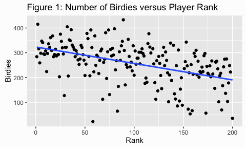
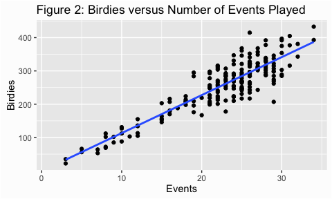
Scatter plots are a useful way to look at the variance of a data and are, typically, our first step in assessing homogeneity. We can illustrate with some golf data provided by ESPN. Here we are assessing the number of birdies players score versus the rank of the player (fig 1) and the number of events played (fig 2). For both figures I added the trend line which makes it easier to assess the variance (or spread of points). In figure 1 it appears that the dots are spread out fairly evenly across the line; this is what is meant by homogeneity of variance.
library(readxl)
library(ggplot2)

golf <- read_excel("Data/Assumptions/Golf Stats.xlsx", sheet = "2011")

ggplot(golf, aes(x = Rank, y = Birdies)) +
        geom_point() +
        geom_smooth(method = "lm", se = FALSE) +
        ggtitle("Figure 1: Number of Birdies versus Player Rank")
In figure 2, however, the variance appears to increase as the number of events played increases. This is an example of heterogeneity of variance, meaning that the variance (or spread) is not consistent across the ranges of values.
ggplot(golf, aes(x = Events, y = Birdies)) +
        geom_point() +
        geom_smooth(method = "lm", se = FALSE) +
        ggtitle("Figure 2: Birdies versus Number of Events Played")
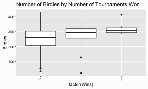
An alternative vizualization is the boxplot. This is commonly used to compare groupings against one-another. In this case we may want to assess how the number of birdies differ among players who have won zero, one, and two tournaments. This plot illustrates that the number of birdies vary widely for players who have no tournament wins. However, players who have one and two tournament wins have an increasing median number of birdies achieved and less variance. This is logical as we would expect players that win more tournaments to have scored more birdies and to be more consistent with the number of birdies scored.
ggplot(golf, aes(x = factor(Wins), y = Birdies)) +
        geom_boxplot() +
        ggtitle("Number of Birdies by Number of Tournaments Won")
Keep in mind that visualizing variance provides indications rather than statistical confirmation of homogeneity (or heterogeneity). To confirm we can perform statistical tests which I cover next.
Bartlett’s test is used to test if k samples are from populations with equal variances; however, Bartlett’s test is sensitive to deviations from normality. If you’ve verified that your data is normally distributed then Bartlett’s test is a good first test but if your data is non-normal than you should always verify results from Bartlett’s test to results from Levene’s and Flinger-Killeen’s tests as there is a good chance you will get a false positive.
When testing one independent variable, such as the variance of birdies across tournament wins we use the bartlett.test() function. For all the tests that follow, the null hypothesis is that all populations variances are equal, the alternative hypothesis is that at least two of them differ. Consequently, p-values less than 0.1, 0.05, 0.001 (depending on your desired threshold) suggest variances are significantly different and the homogeneity of variance assumption has been violated. We can illustrate by testing if the variance in birdies is different among the following groups - zero tournament wins, one win, and two wins.
# feed it data via a data frame
bartlett.test(Birdies ~ Wins, data = golf)
##
## 	Bartlett test of homogeneity of variances
##
## data:  Birdies by Wins
## Bartlett's K-squared = 4.2261, df = 2, p-value = 0.1209

# can also feed it two vectors
bartlett.test(golf$Birdies, golf$Wins)
##
## 	Bartlett test of homogeneity of variances
##
## data:  golf$Birdies and golf$Wins
## Bartlett's K-squared = 4.2261, df = 2, p-value = 0.1209
The Levene’s test is slightly more robust to departures from normality than the Bartlett’s test. Levene’s performs a one-way ANOVA conducted on the deviation scores; that is, the absolute difference between each score and the mean of the group from which it came.1 To test, we use leveneTest() from the car package. By default leveneTest() will test variance around the median but you can override this by using the center = mean argument. In the tests below, we see that both tests have p < 0.1 and the first test (testing variance around the median) has a p < 0.05. This differs from the results from the Bartlett test above, likely because of non-normality in our data.
library(car)

# by default leveneTest will test variance around the median
leveneTest(y = golf$Birdies, group = golf$Wins)
## Levene's Test for Homogeneity of Variance (center = median)
##        Df F value  Pr(>F)
## group   2  3.1417 0.04544 *
##       192
## ---
## Signif. codes:  0 '***' 0.001 '**' 0.01 '*' 0.05 '.' 0.1 ' ' 1

# can override default with center = mean to test variance around the mean
leveneTest(y = golf$Birdies, group = golf$Wins, center = mean)
## Levene's Test for Homogeneity of Variance (center = mean)
##        Df F value  Pr(>F)
## group   2  2.7079 0.06922 .
##       192
## ---
## Signif. codes:  0 '***' 0.001 '**' 0.01 '*' 0.05 '.' 0.1 ' ' 1
As previously stated, Bartlett’s test can provide false positive results when the data is non-normal. Also, when the sample size is large, small differences in group variances can produce a statistically significant Levene’s test (similar to the Shapiro-Wilk test for normality). Fligner-Killeen’s test is a non-parametric test which is robust to departures from normality and provides a good alternative or double check for the previous parametric tests.
fligner.test(Birdies ~ Wins, data = golf)
##
## 	Fligner-Killeen test of homogeneity of variances
##
## data:  Birdies by Wins
## Fligner-Killeen:med chi-squared = 7.7662, df = 2, p-value =
## 0.02059
Similar to the assumption of normality, when we test for violations of constant variance we should not rely on only one approach to assess our data. Rather, we should understand the variance visually and by using multiple testing procedures to come to our conclusion of whether or not homogeneity of variance holds for our data.
See Levene (1960) and Glass (1966) for further discussion. ↩