Fully reproducible approach to turn your analyses into high quality documents, reports, presentations and dashboards.
R Markdown provides an easy way to produce a rich, fully-documented reproducible analysis. It allows the user to share a single file that contains all of the prose, code, and metadata needed to reproduce the analysis from beginning to end. R Markdown allows for “chunks” of R code to be included along with Markdown text to produce a nicely formatted HTML, PDF, or Word file without having to know any HTML or LaTeX code or have to fuss with difficult formatting issues. One R Markdown file can generate a variety of different formats and all of this is done in a single text file with a few bits of formatting.
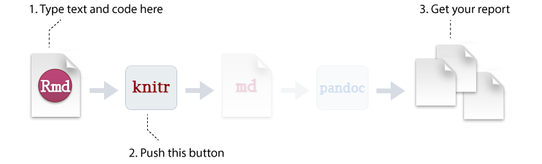
So how does it work? Creating documents with R Markdown starts with an .Rmd file that contains a combination of text and R code chunks. The .Rmd file is fed to knitr, which executes all of the R code chunks and creates a new markdown (.md) document with the output. Pandoc then processes the .md file to create a finished report in the form of a web page, PDF, Word document, slide show, etc.

Sounds confusing you say, don’t fret. Much of what takes place happens behind the scenes. You primarily need to worry only about the syntax required in the .Rmd file. You then press a button and out comes your report.
To create an R Markdown file you can select File » New File » R Markdown or you can select the shortcut for creating a new document in the top left-hand corner of the RStudio window. You will be given an option to create an HTML, PDF, or Word document; however, R Markdown let’s you change seamlessly between these options after you’ve created your document so I tend to just select the default HTML option.
There are additional options such as creating Presentations (HTML or PDF), Shiny documents, or other template documents but for now we will focus on the initial HTML, PDF, or Word document options.
There are three general components of an R Markdown file that you will eventually become accustomed to. This includes the YAML, the general markdown (or text) component, and code chunks.
The first few lines you see in the R Markdown report are known as the YAML.
---
title: "R Markdown Demo"
author: "Brad Boehmke"
date: "2016-08-15"
output: html_document
---
These lines will generate a generic heading at the top of the final report. There are several YAML options to enhance your reports such as the following:
You can include hyperlinks around the title or author name:
---
title: "R Markdown Demo"
author: "[Brad Boehmke](http://bradleyboehmke.github.io)"
date: "2016-08-15"
output: html_document
---
If you don’t want the date to be hard-coded you can include R code so that anytime you re-run the report the current date will print off at the top. You can also exclude the date (or author and title information) by including NULL or simply by deleting that line:
---
title: "R Markdown Demo"
author: "[Brad Boehmke](http://bradleyboehmke.github.io)"
date: "`r Sys.Date()`"
output: html_document
---
By default, your report will not include a table of contents (TOC). However, you can easily generate one by including the toc: true argument. There are several TOC options such as the level of headers to include in the TOC, whether to have a fixed or floating TOC, to have a collapsable TOC, etc. You can find many of the TOC options here.
---
title: "R Markdown Demo"
author: "[Brad Boehmke](http://bradleyboehmke.github.io)"
date: "`r Sys.Date()`"
output:
  html_document:
    toc: true
    toc_float: true
---
When knitr processes an R Markdown input file it creates a markdown (md) file which is subsequently tranformed into HTML by pandoc. If you want to keep a copy of the markdown file after rendering you can do so using the keep_md: true option. This will likely not be a concern at first but when (if) you start doing a lot of online writing you will find that keeping the .md file is extremely beneficial.
---
title: "R Markdown Demo"
author: "[Brad Boehmke](http://bradleyboehmke.github.io)"
date: "`r Sys.Date()`"
output:
  html_document:
    keep_md: true
---
There are many YAML options which you can read more about at:
The beauty of R Markdown is the ability to easily combine prose (text) and code. For the text component, much of your writing is similar to when you type a Word document; however, to perform many of the basic text formatting you use basic markdown code such as:
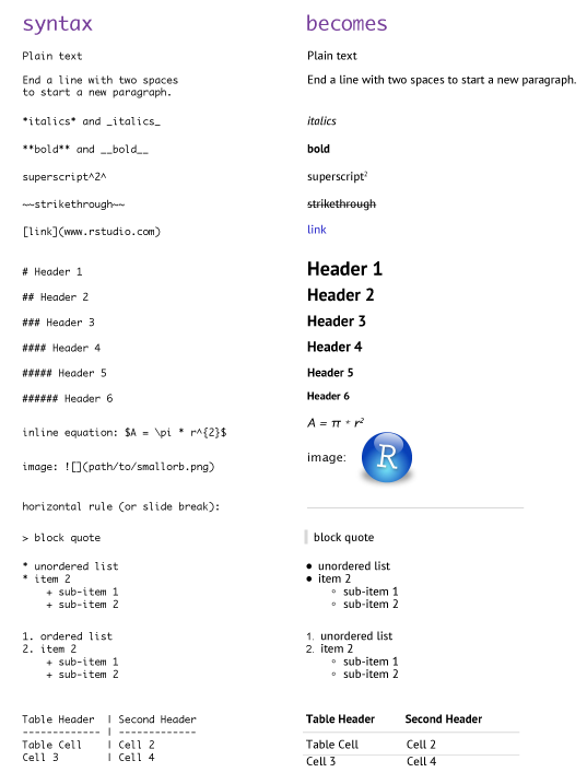
There are many additional formatting options which can be viewed here and here; however, this should get you well on your way.
R code chunks can be used as a means to render R output into documents or to simply display code for illustration. Code chunks start with the following line: ```{r chunk_name} and end with ```. You can quickly insert chunks into your R Markdown file with the keyboard shortcut Cmd + Option + I (Windows Ctrl + Alt + I).
Here is a simple R code chunk that will result in both the code and it’s output being included:
```{r}
head(iris)
```

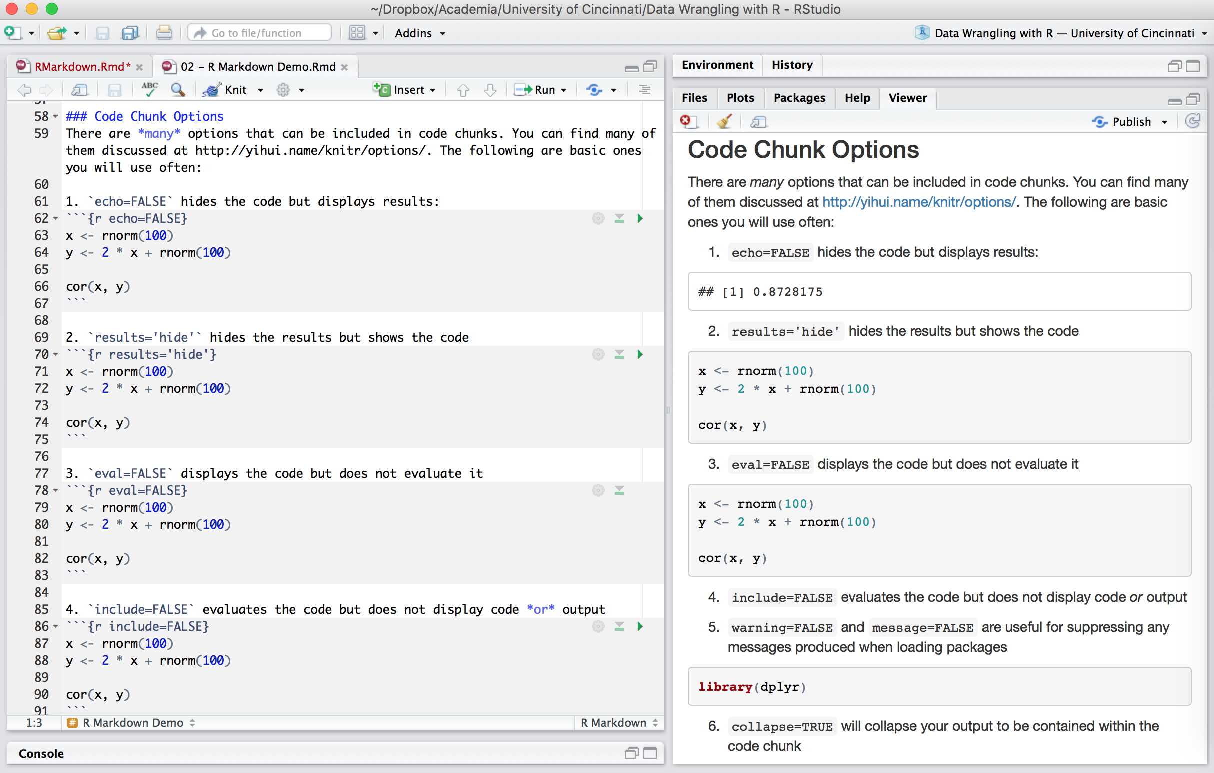
Chunk output can be customized with many knitr options which are arguments set in the {} of a chunk header. Examples include:
1. echo=FALSE hides the code but displays results:
```{r echo=FALSE}
x <- rnorm(100)
y <- 2 * x + rnorm(100)

cor(x, y)
```
2. results='hide' hides the results but shows the code
```{r results='hide'}
x <- rnorm(100)
y <- 2 * x + rnorm(100)

cor(x, y)
```
3. eval=FALSE displays the code but does not evaluate it
```{r eval=FALSE}
x <- rnorm(100)
y <- 2 * x + rnorm(100)

cor(x, y)
```
4. include=FALSE evaluates the code but does not display code or output
```{r include=FALSE}
x <- rnorm(100)
y <- 2 * x + rnorm(100)

cor(x, y)
```
5. warning=FALSE and message=FALSE are useful for suppressing any messages produced when loading packages
```{r, warning=FALSE, message=FALSE}
library(dplyr)
```
6. collapse=TRUE will collapse your output to be contained within the code chunk
```{r, collapse=TRUE}
head(iris)
```
7. fig... options are available to align and size figure outputs
```{r, fig.align='center', fig.height=3, fig.width=4}
library(ggplot2)

ggplot(iris, aes(Sepal.Length, Sepal.Width, color = Species)) +
        geom_point()
```
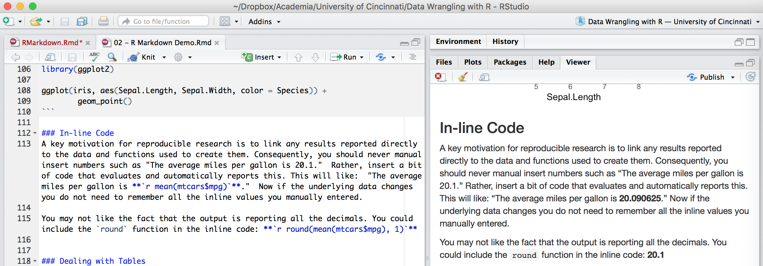
A key motivation for reproducible research is to link any results reported directly to the data and functions used to create them. Consequently, you should never manual insert numbers such as “The average miles per gallon is 20.1.” Rather, code results can be inserted directly into the text of a .Rmd file by enclosing the code with `r ` such as: “The average miles per gallon is `r mean(mtcars$mpg)`.”
Now if the underlying data changes you do not need to remember all the inline values you manually entered. You may not like the fact that the output is reporting all the decimals. You could include the round function in the inline code: `r round(mean(mtcars$mpg), 1)` .
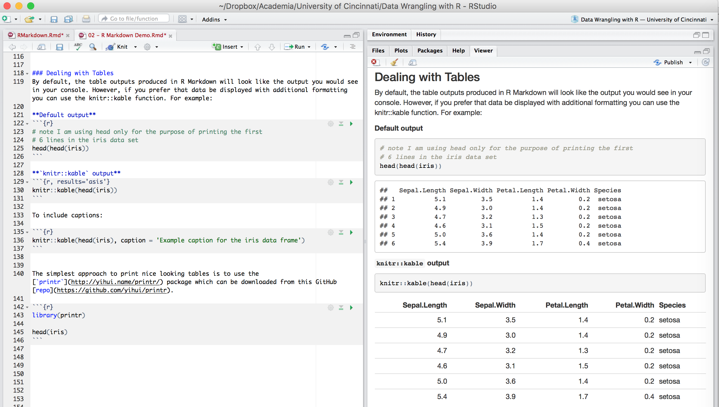
By default, the table outputs produced in R Markdown will look like the output you would see in your console. However, if you prefer that data be displayed with additional formatting you can use the knitr::kable function. For example:
```{r, results='asis'}
knitr::kable(iris)
```
To include captions:
```{r}
knitr::kable(head(iris), caption = 'Example caption for the iris data frame')
```
The simplest approach to print nice looking tables is to use the printr package which can be downloaded from this GitHub repo.
```{r}
library(printr)

head(iris)
```
There are several packages that can be used to make very nice packages:
When you are all done writing your .Rmd document you have two options to render the output. The first is to call the following function in your console: render("document_name.Rmd", output_format = "html_document"). Alternatively you can click the drop down arrow next to the knit button on the RStudio toolbar, select the document format (HTML, PDF, Word) and your report will be developed.
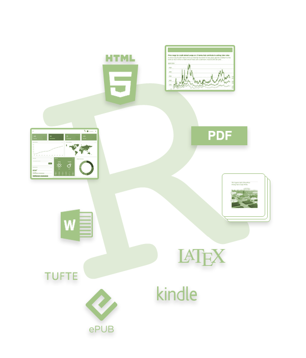
The following output formats are available to use with R Markdown.
R Markdown is an incredible tool for reproducible research and there are a lot of resource available. Here are just a few of the available resources to learn more about R Markdown.
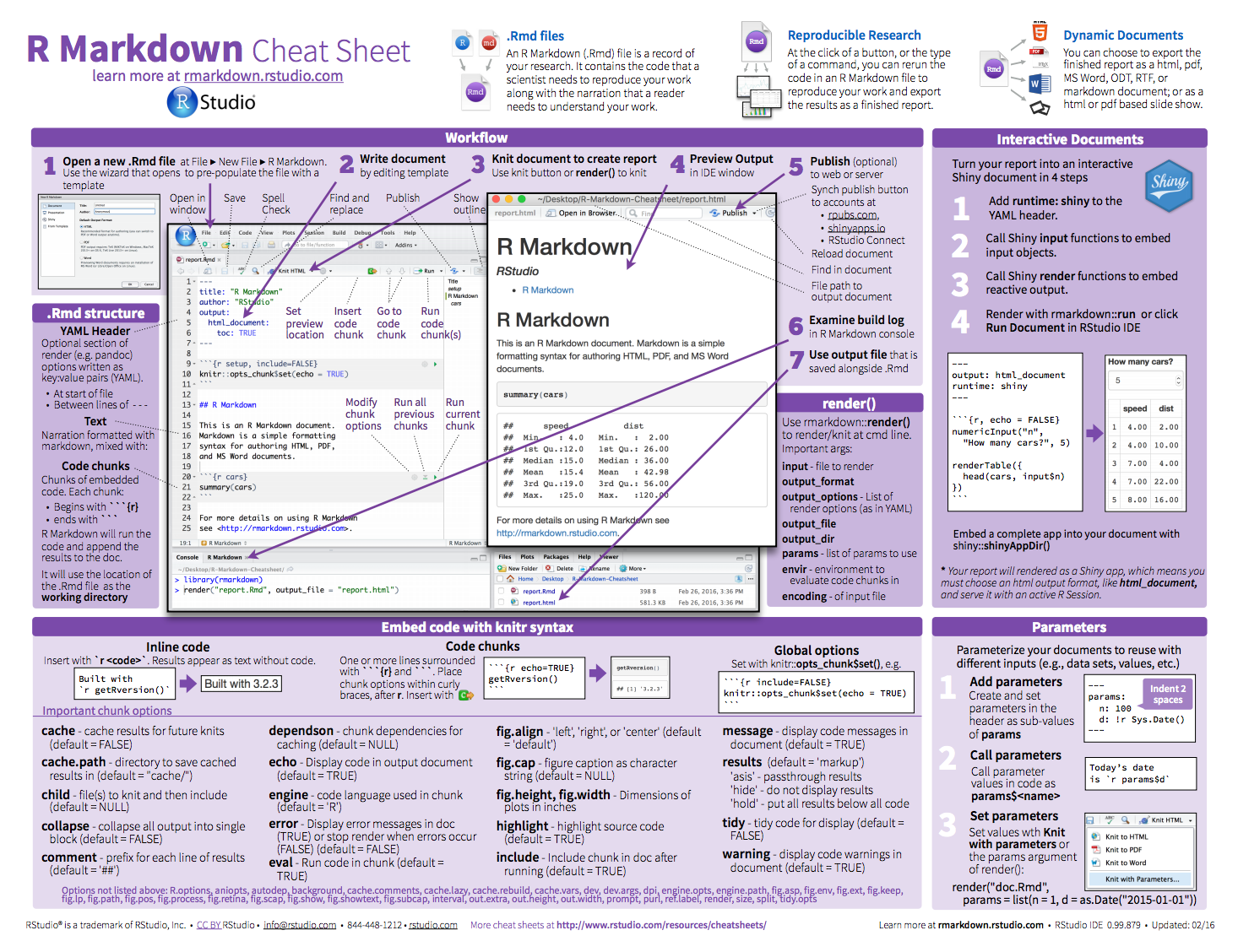
Also, you can find the R Markdown cheatsheet here or within the RStudio console at Help menu » Cheatsheets.