
R is a functional programming language, meaning that everything you do is basically built on functions. However, moving beyond simply using pre-built functions to writing your own functions is when your capabilities really start to take off and your code development/writing takes on a new level of efficiency. Functions allow you to reduce code duplication by automating a generalized task to be applied recursively. Whenever you catch yourself repeating a function or copy and pasting code there is a good change that you should write a function to eliminate the redundancies.
Unfortunately, due to their abstractness, grasping the idea of writing functions (let alone writing them well) can take some time. However, in this section I provide you with the basic knowledge of how functions operate in R to get you started on the right path. To do this, I first outline when you should write functions. I then cover the general components of functions, specifying function arguments, scoping and evaluation rules, managing function outputs, and handling invalid parameters in the Understanding functions section. I then illustrate how you can save & source your own functions for reuse. Lastly, I offer some additional resources that will help you learn more about functions in R.
Note: this section is taken directly from R for Data Science by Garrett Grolemund and Hadley Wickham
You should consider writing a function whenever you’ve copied and pasted a block of code more than twice (i.e. you now have three copies of the same code). For example, take a look at this code. What does it do?
df <- data.frame(
  a = rnorm(10),
  b = rnorm(10),
  c = rnorm(10),
  d = rnorm(10)
)

df$a <- (df$a - min(df$a, na.rm = TRUE)) /
  (max(df$a, na.rm = TRUE) - min(df$a, na.rm = TRUE))
df$b <- (df$b - min(df$b, na.rm = TRUE)) /
  (max(df$a, na.rm = TRUE) - min(df$b, na.rm = TRUE))
df$c <- (df$c - min(df$c, na.rm = TRUE)) /
  (max(df$c, na.rm = TRUE) - min(df$c, na.rm = TRUE))
df$d <- (df$d - min(df$d, na.rm = TRUE)) /
  (max(df$d, na.rm = TRUE) - min(df$d, na.rm = TRUE))
You might be able to puzzle out that this rescales each column to have a range from 0 to 1. But did you spot the mistake? I made an error when copying-and-pasting the code for df$b: I forgot to change an a to a b. Extracting repeated code out into a function is a good idea because it prevents you from making this type of mistake.
To write a function you need to first analyse the code. How many inputs does it have?
(df$a - min(df$a, na.rm = TRUE)) /
  (max(df$a, na.rm = TRUE) - min(df$a, na.rm = TRUE))
This code only has one input: df$a. (It’s a little suprisingly that TRUE is not an input: you can explore why in the exercise below). To make the single input more clear, it’s a good idea to rewrite the code using temporary variables with a general name. Here this function only takes one vector of input, so I’ll call it x:
x <- 1:10
(x - min(x, na.rm = TRUE)) / (max(x, na.rm = TRUE) - min(x, na.rm = TRUE))
##  [1] 0.000 0.111 0.222 0.333 0.444 0.556 0.667 0.778 0.889 1.000
There is some duplication in this code. We’re computing the range of the data three times, but it makes sense to do it in one step:
rng <- range(x, na.rm = TRUE)
(x - rng[1]) / (rng[2] - rng[1])
##  [1] 0.000 0.111 0.222 0.333 0.444 0.556 0.667 0.778 0.889 1.000
Pulling out intermediate calculations into named variables is a good practice because it makes it more clear what the code is doing. Now that I’ve simplified the code, and checked that it still works, I can turn it into a function:
rescale01 <- function(x) {
  rng <- range(x, na.rm = TRUE)
  (x - rng[1]) / (rng[2] - rng[1])
}

rescale01(c(0, 5, 10))
## [1] 0.0 0.5 1.0
To understand functions you need to understand six fundamental items of components:
With the exception of primitive functions all R functions have three parts:
body(): the code inside the functionformals(): the list of arguments used to call the functionenvironment(): the mapping of the location(s) of the function’s variablesFor example, let’s build a function that calculates the present value (PV) of a single future sum. The equation for a single sum PV is: PV = FV/(1+r)n where FV is future value, r is the interest rate, and n is the number of periods. In the function that follows the body of the function includes the equation FV/(1+r)n and then rounding the output to two decimals. The formals (or arguments) required for the function include FV, r, and n. And the environment shows that function operates in the global environment.
PV <- function(FV, r, n) {
        PV <- FV/(1+r)^n
        round(PV, 2)
}

body(PV)
## {
##     PV <- FV/(1 + r)^n
##     round(PV, 2)
## }

formals(PV)
## $FV
##
##
## $r
##
##
## $n

environment(PV)
## <environment: R_GlobalEnv>
To perform the PV() function we can call the arguments in different ways.
# using argument names
PV(FV = 1000, r = .08, n = 5)
## [1] 680.58

# same as above but without using names (aka "positional matching")
PV(1000, .08, 5)
## [1] 680.58

# if using names you can change the order
PV(r = .08, FV = 1000, n = 5)
## [1] 680.58

# if not using names you must insert arguments in proper order
# in this e.g. the function assumes FV = .08, r = 1000, and n = 5
PV(.08, 1000, 5)
## [1] 0
Note that when building a function you can also set default values for arguments. In our original PV() we did not provide any default values so if we do not supply all the argument parameters an error will be returned. However, if we set default values then the function will use the stated default if any parameters are missing:
# missing the n argument
PV(1000, .08)
## Error in PV(1000, 0.08): argument "n" is missing, with no default

# creating default argument values
PV <- function(FV = 1000, r = .08, n = 5) {
        PV <- FV/(1+r)^n
        round(PV, 2)
}

# function will use default n value
PV(1000, .08)
## [1] 680.58

# specifying a different n value
PV(1000, .08, 3)
## [1] 793.83
Scoping refers to the set of rules a programming language uses to lookup the value to variables and/or symbols. The following illustrates the basic concept behind the lexical scoping rules that R follows.
A function will first look inside the function to identify all the variables being called. If all variables exist then their is no additional search required to identify variables.
PV1 <- function() {
        FV <- 1000
        r <- .08
        n <- 5
        FV/(1+r)^n
}

PV1()
## [1] 680.5832
However, if a variable does not exist within the function, R will look one level up to see if the variable exists.
# the FV variable is outside the function environment
FV <- 1000

PV2 <- function() {
        r <- .08
        n <- 5
        FV/(1+r)^n
}

PV2()
## [1] 680.5832
This same concept applies if you have functions embeded within functions:
FV <- 1000

PV3 <- function() {
        r <- .08
        n <- 5
        denominator <- function() {
                (1+r)^n
        }
        FV/denominator()
}

PV3()
## [1] 680.5832
This also applies for functions in which some arguments are called but not all variables used in the body are identified as arguments:
# n is specified within the function
PV4 <- function(FV, r) {
        n <- 5
        FV/(1+r)^n
}

PV4(1000, .08)
## [1] 680.5832

# n is specified within the function and
# r is specified outside the function
r <- 0.08

PV5 <- function(FV) {
        n <- 5
        FV/(1+r)^n
}

PV5(1000)
## [1] 680.5832
R functions perform “lazy” evaluation in which arguments are only evaluated if required in the body of the function.
# the y argument is not used so not included it causes
# no harm
lazy <- function(x, y){
        x*2
}
lazy(4)
## [1] 8

# however, if both arguments are required in the body
# an error will result if an argument is missing
lazy2 <- function(x, y){
        (x+y)*2
}
lazy2(4)
## Error in lazy2(4): argument "y" is missing, with no default
If a function performs multiple tasks and therefore has multiple results to report then we have to include the c() function inside the function to display all the results. If you do not include the c() function then the function output will only return the last expression:
bad <- function(x, y) {
        2*x + y
        x + 2*y
        2*x + 2*y
        x/y
}
bad(1, 2)
## [1] 0.5

good <- function(x, y) {
        output1 <- 2*x + y
        output2 <- x + 2*y
        output3 <- 2*x + 2*y
        output4 <- x/y
        c(output1, output2, output3, output4)
}
good(1, 2)
## [1] 4.0 5.0 6.0 0.5
Furthermore, when we have a function which performs multiple tasks (i.e. computes multiple computations) then it is often useful to save the results in a list.
good_list <- function(x, y) {
        output1 <- 2*x + y
        output2 <- x + 2*y
        output3 <- 2*x + 2*y
        output4 <- x/y
        c(list(Output1 = output1, Output2 = output2,
               Output3 = output3, Output4 = output4))
}
good_list(1, 2)
## $Output1
## [1] 4
##
## $Output2
## [1] 5
##
## $Output3
## [1] 6
##
## $Output4
## [1] 0.5
For functions that will be used again, and especially for those used by someone other than the creator of the function, it is good to check the validity of arguments within the function. One way to do this is to use the stop() function. The following uses an if() statement to check if the class of each argument is numeric. If one or more arguments are not numeric then the stop() function will be triggered to provide a meaning message to the user.
PV <- function(FV, r, n) {
        if(!is.numeric(FV) | !is.numeric(r) | !is.numeric(n)){
                stop('This function only works for numeric inputs!\n',
                     'You have provided objects of the following classes:\n',
                     'FV: ', class(FV), '\n',
                     'r: ', class(r), '\n',
                     'n: ', class(n))
        }

        PV <- FV/(1+r)^n
        round(PV, 2)
}

PV("1000", 0.08, "5")
## Error in PV("1000", 0.08, "5"): This function only works for numeric inputs!
## You have provided objects of the following classes:
## FV: character
## r: numeric
## n: character
Another concern is dealing with missing or NA values. Lets say you wanted to perform the PV() function on a vector of potential future values. The function as is will output NA in place of any missing values in the FV input vector. If you want to remove the missing values then you can incorporate the na.rm parameter in the function arguments along with an if statement to remove missing values if na.rm = TRUE.
# vector of future value inputs
fv <- c(800, 900, NA, 1100, NA)

PV(fv, .08, 5)
## [1] 544.47 612.52     NA 748.64     NA

PV <- function(FV, r, n, na.rm = FALSE) {
        if(!is.numeric(FV) | !is.numeric(r) | !is.numeric(n)){
                stop('This function only works for numeric inputs!\n',
                     'You have provided objects of the following classes:\n',
                     'FV: ', class(FV), '\n',
                     'r: ', class(r), '\n',
                     'n: ', class(n))
        }

        if(na.rm == TRUE) {
                FV <- FV[!is.na(FV)]
        }

        PV <- FV/(1+r)^n
        round(PV, 2)
}

PV(fv, 0.08, 5, na.rm = TRUE)
## [1] 544.47 612.52 748.64
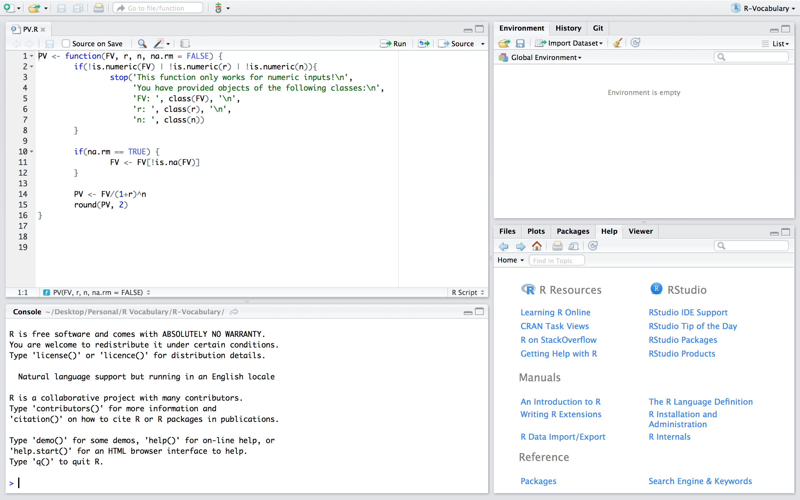
If you want to save a function to be used at other times and within other scripts there are two main ways to do this. One way is to build a package which is discussed in more details here. Another option, and the one discussed here, is to save the function in a script. For example, we can save a script that contains the PV() function from the previous section and save this script as PV.R.
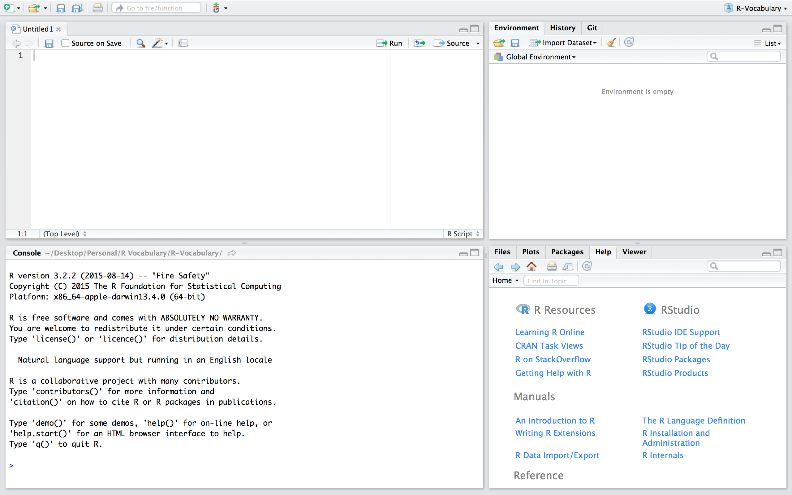
Now, if we are working in a fresh script you’ll see that we have no objects and functions in our working environment:
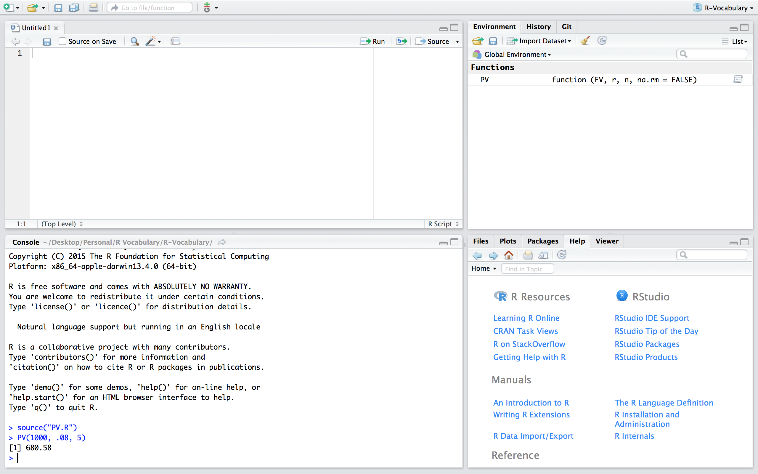
If we want to use the PV function in this new script we can simply read in the function by sourcing the script using source("PV.R"). Now, you’ll notice that we have the PV() function in our global environment and can use it as normal. Note that if you are working in a different directory then where the PV.R file is located you’ll need to include the proper command to access the relevant directory.
Functions are a fundamental building block of R and writing functions is a core activity of an R programmer. It represents the key step of the transition from a mere “user” to a developer who creates new functionality for R. As a result, its important to turn your existing, informal knowledge of functions into a rigorous understanding of what functions are and how they work. A few additional resources that can help you get to the next step of understanding functions include: