
Rapid growth of the World Wide Web has significantly changed the way we share, collect, and publish data. Vast amount of information is being stored online, both in structured and unstructured forms. Regarding certain questions or research topics, this has resulted in a new problem - no longer is the concern of data scarcity and inaccessibility but, rather, one of overcoming the tangled masses of online data.
Collecting data from the web is not an easy process as there are many technologies used to distribute web content (i.e. HTML, XML, JSON). Therefore, dealing with more advanced web scraping requires familiarity in accessing data stored in these technologies via R. Through this section I will provide an introduction to some of the fundamental tools required to perform basic web scraping. This includes importing spreadsheet data files stored online, scraping HTML text, scraping HTML table data, and leveraging APIs to scrape data.
My purpose in the following sections is to discuss these topics at a level meant to get you started in web scraping; however, this area is vast and complex and this chapter will far from provide you expertise level insight. To advance your knowledge I highly recommend getting copies of XML and Web Technologies for Data Sciences with R and Automated Data Collection with R.
Note: the examples provided below were performed in 2015. Consequently, if you apply the code provide throughout these examples your outputs may differ due to webpages and their content changing over time.
The most basic form of getting data from online is to import tabular (i.e. .txt, .csv) or Excel files that are being hosted online. This is often not considered web scraping1; however, I think its a good place to start introducing the user to interacting with the web for obtaining data. Importing tabular data is especially common for the many types of government data available online. A quick perusal of Data.gov illustrates over 190,000 examples. In fact, we can provide our first example of importing online tabular data by downloading the Data.gov .csv file that lists all the federal agencies that supply data to Data.gov.
# the url for the online CSV
url <- "https://s3.amazonaws.com/bsp-ocsit-prod-east-appdata/datagov/wordpress/agency-participation.csv"

# use read.csv to import
data_gov <- read.csv(url, stringsAsFactors = FALSE)

# for brevity I only display first 6 rows
head(data_gov)
##                                      Agency.Name                 Sub.Agency.Publisher Organization.Type Datasets Last.Entry
## 1                Broadcasting Board of Governors                                          Federal-Other        6 01/12/2014
## 2           Commodity Futures Trading Commission                                          Federal-Other        3 01/12/2014
## 3           Consumer Financial Protection Bureau                                          Federal-Other        2 09/26/2015
## 4           Consumer Financial Protection Bureau Consumer Financial Protection Bureau     Federal-Other        2 09/26/2015
## 5 Corporation for National and Community Service                                          Federal-Other        3 01/12/2014
## 6 Court Services and Offender Supervision Agency                                          Federal-Other        1 01/12/2014
Downloading Excel spreadsheets hosted online can be performed just as easily. Recall that there is not a base R function for importing Excel data; however, several packages exist to handle this capability. One package that works smoothly with pulling Excel data from urls is gdata. With gdata we can use read.xls() to download this Fair Market Rents for Section 8 Housing Excel file from the given url.
library(gdata)

# the url for the online Excel file
url <- "http://www.huduser.org/portal/datasets/fmr/fmr2015f/FY2015F_4050_Final.xls"

# use read.xls to import
rents <- read.xls(url)

rents[1:6, 1:10]
##    fips2000  fips2010 fmr2 fmr0 fmr1 fmr3 fmr4 county State CouSub
## 1 100199999 100199999  788  628  663 1084 1288      1     1  99999
## 2 100399999 100399999  762  494  643 1123 1318      3     1  99999
## 3 100599999 100599999  670  492  495  834  895      5     1  99999
## 4 100799999 100799999  773  545  652 1015 1142      7     1  99999
## 5 100999999 100999999  773  545  652 1015 1142      9     1  99999
## 6 101199999 101199999  599  481  505  791 1061     11     1  99999
Note that many of the arguments covered in the Importing Data section (i.e. specifying sheets to read from, skipping lines) also apply to read.xls(). In addition, gdata provides some useful functions (sheetCount() and sheetNames()) for identifying if multiple sheets exist prior to downloading. Check out ?gdata for more help.
Special note when using gdata on Windows: When downloading excel spreadsheets from the internet, Mac users will be able to install the gdata package, attach the library, and be highly functional right away. Windows users, on the other hand, do not have a Perl interpreter installed by default.
install.packages("gdata")
If you are a Windows user and attempt to attach the gdata library immediately after installation, you will likely receive the warning message given in Figure 1. You will not be able to download excel spreadsheets from the internet without installing some additional software.
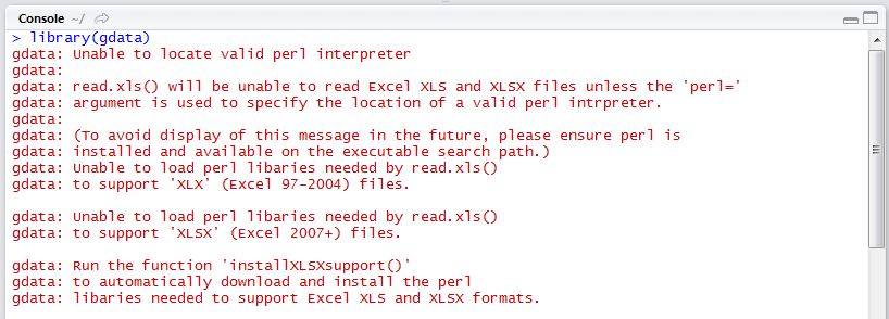
gdata without Perl
Unfortunately, it’s not as straightforward to fix as the error message would indicate. Running installXLSXsupport() won’t completely solve your problem without Perl software installed. In order for gdata to function properly, you must install ActiveState Perl using the following link: http://www.activestate.com/activeperl/. The download could take up to 10 minutes or so, and when finished, you will need to find where the software was stored on your machine (likely directly on the C:/ Drive).
Once Perl software has been installed, you will need to direct R to find it each time you call the function.
# use read.xls to import
rents <- read.xls(url, perl = "C:/Perl64/bin/perl.exe")
Another common form of file storage is using zip files. For instance, the Bureau of Labor Statistics (BLS) stores their public-use microdata for the Consumer Expenditure Survey in .zip files. We can use download.file() to download the file to your working directory and then work with this data as desired.
url <- "http://www.bls.gov/cex/pumd/data/comma/diary14.zip"

# download .zip file and unzip contents
download.file(url, dest = "dataset.zip", mode = "wb")
unzip("dataset.zip", exdir = "./")

# assess the files contained in the .zip file which
# unzips as a folder named "diary14"
list.files("diary14")
##  [1] "dtbd141.csv" "dtbd142.csv" "dtbd143.csv" "dtbd144.csv" "dtid141.csv"
##  [6] "dtid142.csv" "dtid143.csv" "dtid144.csv" "expd141.csv" "expd142.csv"
## [11] "expd143.csv" "expd144.csv" "fmld141.csv" "fmld142.csv" "fmld143.csv"
## [16] "fmld144.csv" "memd141.csv" "memd142.csv" "memd143.csv" "memd144.csv"

# alternatively, if we know the file we want prior to unzipping
# we can extract the file without unzipping using unz():
zip_data <- read.csv(unz("dataset.zip", "diary14/expd141.csv"))
zip_data[1:5, 1:10]
##     NEWID ALLOC COST GIFT PUB_FLAG    UCC EXPNSQDY EXPN_QDY EXPNWKDY   EXPN_KDY
## 1 2825371     0 6.26    2        2 190112        1        D        3        D
## 2 2825371     0 1.20    2        2 190322        1        D        3        D
## 3 2825381     0 0.98    2        2  20510        3        D        2        D
## 4 2825381     0 0.98    2        2  20510        3        D        2        D
## 5 2825381     0 2.50    2        2  20510        3        D        2        D
The .zip archive file format is meant to compress files and are typically used on files of significant size. For instance, the Consumer Expenditure Survey data we downloaded in the previous example is over 10MB. Obviously there may be times in which we want to get specific data in the .zip file to analyze but not always permanently store the entire .zip file contents. In these instances we can use the following process proposed by Dirk Eddelbuettel to temporarily download the .zip file, extract the desired data, and then discard the .zip file.
# Create a temp. file name
temp <- tempfile()

# Use download.file() to fetch the file into the temp. file
download.file("http://www.bls.gov/cex/pumd/data/comma/diary14.zip",temp)

# Use unz() to extract the target file from temp. file
zip_data2 <- read.csv(unz(temp, "diary14/expd141.csv"))

# Remove the temp file via unlink()
unlink(temp)

zip_data2[1:5, 1:10]
##     NEWID ALLOC COST GIFT PUB_FLAG    UCC EXPNSQDY EXPN_QDY EXPNWKDY   EXPN_KDY
## 1 2825371     0 6.26    2        2 190112        1        D        3        D
## 2 2825371     0 1.20    2        2 190322        1        D        3        D
## 3 2825381     0 0.98    2        2  20510        3        D        2        D
## 4 2825381     0 0.98    2        2  20510        3        D        2        D
## 5 2825381     0 2.50    2        2  20510        3        D        2        D
One last common scenario I’ll cover when importing spreadsheet data from online is when we identify multiple data sets that we’d like to download but are not centrally stored in a single .zip format or the like. For example there are multiple data files scattered throughout the Maryland State Board of Elections website that we may want to download. The first objective here is to identify the relevant links. The XML package provides the useful getHTMLLinks() function to identify these links.
library(XML)

url <- "http://www.elections.state.md.us/elections/2012/election_data/index.html"
links <- getHTMLLinks(url)
head(links)
## [1] "http://www.maryland.gov/"
## [2] "../../../index.html"
## [3] "../../../index.html"
## [4] "https://www.facebook.com/MarylandStateBoardofElections"
## [5] "https://twitter.com/md_sbe"
## [6] "http://www.maryland.gov/pages/social_media.aspx"
However, this provides all the links on the page. For this example we will only concentrate on the links that contain .csv files. Here, we see that there are 307 .csv files.
library(stringr)

# extract names for desired links and paste to url
links_data <- links[str_detect(links, ".csv")]

length(links_data)
## [1] 307
If we wanted to we could loop through and download all 307 .csv files. However, for simplicity we’ll just download the first six files and save each one as a separate data frame.
links_data <- head(links_data)

for(i in seq_along(links_data)) {

  # step 1: paste .csv portion of link to the base URL
  url <- paste0("http://www.elections.state.md.us/elections/2012/election_data/",
                links_data[i])

  # step 2: download .csv file and save as df
  df <- read.csv(url)

  # step 3: rename df
  assign(paste0("df", i), df)
}
I now have the six downloaded data frames in my global environment saved as “df1”, “df2”, “df3”, “df4”, “df5”, and “df6”
sapply(paste0("df", 1:6), exists)
##  df1  df2  df3  df4  df5  df6
## TRUE TRUE TRUE TRUE TRUE TRUE

head(df1)
##   County                            Candidate.Name Party             Office.Name Office.District Winner CONG.08 CONG.04 CONG.07 CONG.01 CONG.03 CONG.02 CONG.05 CONG.06
## 1      0                              Barack Obama   DEM   President - Vice Pres                      Y   30138   37385   38838   15734   26963   22444   34224   26702
## 2      0 Uncommitted To Any Presidential Candidate   DEM   President - Vice Pres                           3186    1815    2797    6007    4959    4408    3640    4991
## 3      0                      Raymond Levi Blagmon   DEM U.S. Senator                                       443     662     672     568     646     594     589     786
## 4      0                                Ben Cardin   DEM U.S. Senator                                 Y   28493   22818   31357   16589   25800   20669   23218   24589
## 5      0                              J. P. Cusick   DEM U.S. Senator                                       350     229     387     686     526     562     612     713
## 6      0                              Chris Garner   DEM U.S. Senator                                       976     694     733    1232     829     838     961    1577
These examples provide the basics required for downloading most tabular and Excel files from online. However, this is just the beginning of importing/scraping data from the web. Next, we’ll start exploring the more conventional forms of scraping text and data stored in HTML webpages.
Vast amount of information exists across the interminable webpages that exist online. Much of this information are “unstructured” text that may be useful in our analyses. This section covers the basics of scraping these texts from online sources. Throughout this section I will illustrate how to extract different text components of webpages by dissecting the Wikipedia page on web scraping. However, its important to first cover one of the basic components of HTML elements as we will leverage this information to pull desired information. I offer only enough insight required to begin scraping; I highly recommend XML and Web Technologies for Data Sciences with R and Automated Data Collection with R to learn more about HTML and XML element structures.
HTML elements are written with a start tag, an end tag, and with the content in between: <tagname>content</tagname>. The tags which typically contain the textual content we wish to scrape, and the tags we will leverage in the next two sections, include:
<h1>, <h2>,…,<h6>: Largest heading, second largest heading, etc.<p>: Paragraph elements<ul>: Unordered bulleted list<ol>: Ordered list<li>: Individual List item<div>: Division or section<table>: TableFor example, text in paragraph form that you see online is wrapped with the HTML paragraph tag <p> as in:
<p>
This paragraph represents
a typical text paragraph
in HTML form
</p>
It is through these tags that we can start to extract textual components (also referred to as nodes) of HTML webpages.
To scrape online text we’ll make use of the relatively newer rvest package. rvest was created by the RStudio team inspired by libraries such as beautiful soup which has greatly simplified web scraping. rvest provides multiple functionalities; however, in this section we will focus only on extracting HTML text with rvest. Its important to note that rvest makes use of of the pipe operator (%>%) developed through the magrittr package. If you are not familiar with the functionality of %>% I recommend you jump to the section on Simplifying Your Code with %>% so that you have a better understanding of what’s going on with the code.
To extract text from a webpage of interest, we specify what HTML elements we want to select by using html_nodes(). For instance, if we want to scrape the primary heading for the Web Scraping Wikipedia webpage we simply identify the <h1> node as the node we want to select. html_nodes() will identify all <h1> nodes on the webpage and return the HTML element. In our example we see there is only one <h1> node on this webpage.
library(rvest)

scraping_wiki <- read_html("https://en.wikipedia.org/wiki/Web_scraping")

scraping_wiki %>%
        html_nodes("h1")
## {xml_nodeset (1)}
## [1] <h1 id="firstHeading" class="firstHeading" lang="en">Web scraping</h1>
To extract only the heading text for this <h1> node, and not include all the HTML syntax we use html_text() which returns the heading text we see at the top of the Web Scraping Wikipedia page.
scraping_wiki %>%
        html_nodes("h1") %>%
        html_text()
## [1] "Web scraping"
If we want to identify all the second level headings on the webpage we follow the same process but instead select the <h2> nodes. In this example we see there are 10 second level headings on the Web Scraping Wikipedia page.
scraping_wiki %>%
        html_nodes("h2") %>%
        html_text()
##  [1] "Contents"
##  [2] "Techniques[edit]"
##  [3] "Legal issues[edit]"
##  [4] "Notable tools[edit]"
##  [5] "See also[edit]"
##  [6] "Technical measures to stop bots[edit]"
##  [7] "Articles[edit]"
##  [8] "References[edit]"
##  [9] "See also[edit]"
## [10] "Navigation menu"
Next, we can move on to extracting much of the text on this webpage which is in paragraph form. We can follow the same process illustrated above but instead we’ll select all <p> nodes. This selects the 17 paragraph elements from the web page; which we can examine by subsetting the list p_nodes to see the first line of each paragraph along with the HTML syntax. Just as before, to extract the text from these nodes and coerce them to a character string we simply apply html_text().
p_nodes <- scraping_wiki %>%
        html_nodes("p")

length(p_nodes)
## [1] 17

p_nodes[1:6]
## {xml_nodeset (6)}
## [1] <p><b>Web scraping</b> (<b>web harvesting</b> or <b>web data extract ...
## [2] <p>Web scraping is closely related to <a href="/wiki/Web_indexing" t ...
## [3] <p/>
## [4] <p/>
## [5] <p>Web scraping is the process of automatically collecting informati ...
## [6] <p>Web scraping may be against the <a href="/wiki/Terms_of_use" titl ...


p_text <- scraping_wiki %>%
        html_nodes("p") %>%
        html_text()

p_text[1]
## [1] "Web scraping (web harvesting or web data extraction) is a computer software technique of extracting information from websites. Usually, such software programs simulate human exploration of the World Wide Web by either implementing low-level Hypertext Transfer Protocol (HTTP), or embedding a fully-fledged web browser, such as Mozilla Firefox."
Not too bad; however, we may not have captured all the text that we were hoping for. Since we extracted text for all <p> nodes, we collected all identified paragraph text; however, this does not capture the text in the bulleted lists. For example, when you look at the Web Scraping Wikipedia page you will notice a significant amount of text in bulleted list format following the third paragraph under the Techniques heading. If we look at our data we’ll see that that the text in this list format are not capture between the two paragraphs:
p_text[5]
## [1] "Web scraping is the process of automatically collecting information from the World Wide Web. It is a field with active developments sharing a common goal with the semantic web vision, an ambitious initiative that still requires breakthroughs in text processing, semantic understanding, artificial intelligence and human-computer interactions. Current web scraping solutions range from the ad-hoc, requiring human effort, to fully automated systems that are able to convert entire web sites into structured information, with limitations."

p_text[6]
## [1] "Web scraping may be against the terms of use of some websites. The enforceability of these terms is unclear.[4] While outright duplication of original expression will in many cases be illegal, in the United States the courts ruled in Feist Publications v. Rural Telephone Service that duplication of facts is allowable. U.S. courts have acknowledged that users of \"scrapers\" or \"robots\" may be held liable for committing trespass to chattels,[5][6] which involves a computer system itself being considered personal property upon which the user of a scraper is trespassing. The best known of these cases, eBay v. Bidder's Edge, resulted in an injunction ordering Bidder's Edge to stop accessing, collecting, and indexing auctions from the eBay web site. This case involved automatic placing of bids, known as auction sniping. However, in order to succeed on a claim of trespass to chattels, the plaintiff must demonstrate that the defendant intentionally and without authorization interfered with the plaintiff's possessory interest in the computer system and that the defendant's unauthorized use caused damage to the plaintiff. Not all cases of web spidering brought before the courts have been considered trespass to chattels.[7]"
This is because the text in this list format are contained in <ul> nodes. To capture the text in lists, we can use the same steps as above but we select specific nodes which represent HTML lists components. We can approach extracting list text two ways.
First, we can pull all list elements (<ul>). When scraping all <ul> text, the resulting data structure will be a character string vector with each element representing a single list consisting of all list items in that list. In our running example there are 21 list elements as shown in the example that follows. You can see the first list scraped is the table of contents and the second list scraped is the list in the Techniques section.
ul_text <- scraping_wiki %>%
        html_nodes("ul") %>%
        html_text()

length(ul_text)
## [1] 21

ul_text[1]
## [1] "\n1 Techniques\n2 Legal issues\n3 Notable tools\n4 See also\n5 Technical measures to stop bots\n6 Articles\n7 References\n8 See also\n"

# read the first 200 characters of the second list
substr(ul_text[2], start = 1, stop = 200)
## [1] "\nHuman copy-and-paste: Sometimes even the best web-scraping technology cannot replace a human’s manual examination and copy-and-paste, and sometimes this may be the only workable solution when the web"
An alternative approach is to pull all <li> nodes. This will pull the text contained in each list item for all the lists. In our running example there’s 146 list items that we can extract from this Wikipedia page. The first eight list items are the list of contents we see towards the top of the page. List items 9-17 are the list elements contained in the “Techniques” section, list items 18-44 are the items listed under the “Notable Tools” section, and so on.
li_text <- scraping_wiki %>%
        html_nodes("li") %>%
        html_text()

length(li_text)
## [1] 147

li_text[1:8]
## [1] "1 Techniques"                      "2 Legal issues"
## [3] "3 Notable tools"                   "4 See also"
## [5] "5 Technical measures to stop bots" "6 Articles"
## [7] "7 References"                      "8 See also"
At this point we may believe we have all the text desired and proceed with joining the paragraph (p_text) and list (ul_text or li_text) character strings and then perform the desired textual analysis. However, we may now have captured more text than we were hoping for. For example, by scraping all lists we are also capturing the listed links in the left margin of the webpage. If we look at the 104-136 list items that we scraped, we’ll see that these texts correspond to the left margin text.
li_text[104:136]
##  [1] "Main page"           "Contents"            "Featured content"
##  [4] "Current events"      "Random article"      "Donate to Wikipedia"
##  [7] "Wikipedia store"     "Help"                "About Wikipedia"
## [10] "Community portal"    "Recent changes"      "Contact page"
## [13] "What links here"     "Related changes"     "Upload file"
## [16] "Special pages"       "Permanent link"      "Page information"
## [19] "Wikidata item"       "Cite this page"      "Create a book"
## [22] "Download as PDF"     "Printable version"   "Català"
## [25] "Deutsch"             "Español"             "Français"
## [28] "Íslenska"            "Italiano"            "Latviešu"
## [31] "Nederlands"          "日本語"              "Српски / srpski"
If we desire to scrape every piece of text on the webpage than this won’t be of concern. In fact, if we want to scrape all the text regardless of the content they represent there is an easier approach. We can capture all the content to include text in paragraph (<p>), lists (<ul>, <ol>, and <li>), and even data in tables (<table>) by using <div>. This is because these other elements are usually a subsidiary of an HTML division or section so pulling all <div> nodes will extract all text contained in that division or section regardless if it is also contained in a paragraph or list.
all_text <- scraping_wiki %>%
        html_nodes("div") %>%
        html_text()
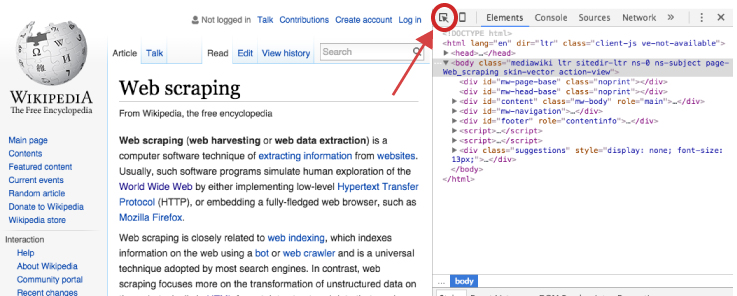
However, if we are concerned only with specific content on the webpage then we need to make our HTML node selection process a little more focused. To do this we, we can use our browser’s developer tools to examine the webpage we are scraping and get more details on specific nodes of interest. If you are using Chrome or Firefox you can open the developer tools by clicking F12 (Cmd + Opt + I for Mac) or for Safari you would use Command-Option-I. An additional option which is recommended by Hadley Wickham is to use selectorgadget.com, a Chrome extension, to help identify the web page elements you need2.
Once the developer’s tools are opened your primary concern is with the element selector. This is located in the top lefthand corner of the developers tools window.
Once you’ve selected the element selector you can now scroll over the elements of the webpage which will cause each element you scroll over to be highlighted. Once you’ve identified the element you want to focus on, select it. This will cause the element to be identified in the developer tools window. For example, if I am only interested in the main body of the Web Scraping content on the Wikipedia page then I would select the element that highlights the entire center component of the webpage. This highlights the corresponding element <div id="bodyContent" class="mw-body-content"> in the developer tools window as the following illustrates.
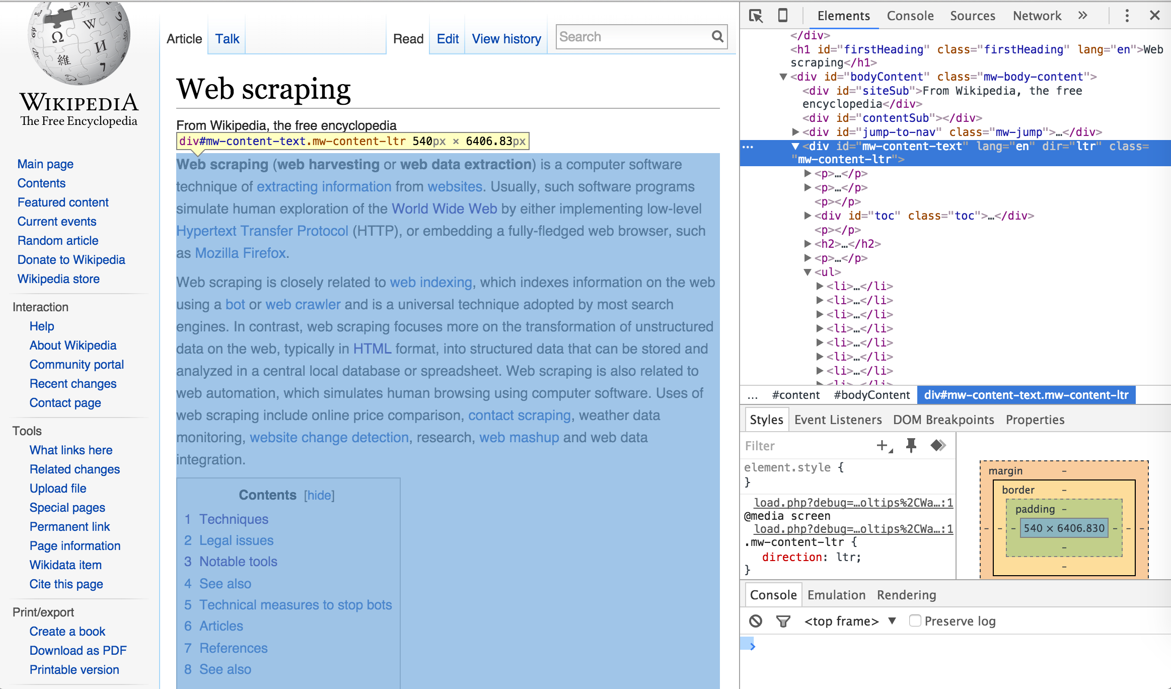
I can now use this information to select and scrape all the text from this specific <div> node by calling the ID name (“#mw-content-text”) in html_nodes()3. As you can see below, the text that is scraped begins with the first line in the main body of the Web Scraping content and ends with the text in the See Also section which is the last bit of text directly pertaining to Web Scraping on the webpage. Explicitly, we have pulled the specific text associated with the web content we desire.
body_text <- scraping_wiki %>%
        html_nodes("#mw-content-text") %>%
        html_text()

# read the first 207 characters
substr(body_text, start = 1, stop = 207)
## [1] "Web scraping (web harvesting or web data extraction) is a computer software technique of extracting information from websites. Usually, such software programs simulate human exploration of the World Wide Web"

# read the last 73 characters
substr(body_text, start = nchar(body_text)-73, stop = nchar(body_text))
## [1] "See also[edit]\n\nData scraping\nData wrangling\nKnowledge extraction\n\n\n\n\n\n\n\n\n"
Using the developer tools approach allows us to be as specific as we desire. We can identify the class name for a specific HTML element and scrape the text for only that node rather than all the other elements with similar tags. This allows us to scrape the main body of content as we just illustrated or we can also identify specific headings, paragraphs, lists, and list components if we desire to scrape only these specific pieces of text:
# Scraping a specific heading
scraping_wiki %>%
        html_nodes("#Techniques") %>%
        html_text()
## [1] "Techniques"

# Scraping a specific paragraph
scraping_wiki %>%
        html_nodes("#mw-content-text > p:nth-child(20)") %>%
        html_text()
## [1] "In Australia, the Spam Act 2003 outlaws some forms of web harvesting, although this only applies to email addresses.[20][21]"

# Scraping a specific list
scraping_wiki %>%
        html_nodes("#mw-content-text > div:nth-child(22)") %>%
        html_text()
## [1] "\n\nApache Camel\nArchive.is\nAutomation Anywhere\nConvertigo\ncURL\nData Toolbar\nDiffbot\nFirebug\nGreasemonkey\nHeritrix\nHtmlUnit\nHTTrack\niMacros\nImport.io\nJaxer\nNode.js\nnokogiri\nPhantomJS\nScraperWiki\nScrapy\nSelenium\nSimpleTest\nwatir\nWget\nWireshark\nWSO2 Mashup Server\nYahoo! Query Language (YQL)\n\n"

# Scraping a specific reference list item
scraping_wiki %>%
        html_nodes("#cite_note-22") %>%
        html_text()
## [1] "^ \"Web Scraping: Everything You Wanted to Know (but were afraid to ask)\". Distil Networks. 2015-07-22. Retrieved 2015-11-04. "
With any webscraping activity, especially involving text, there is likely to be some clean up involved. For example, in the previous example we saw that we can specifically pull the list of Notable Tools; however, you can see that in between each list item rather than a space there contains one or more \n which is used in HTML to specify a new line. We can clean this up quickly with a little character string manipulation.
library(magrittr)

scraping_wiki %>%
        html_nodes("#mw-content-text > div:nth-child(22)") %>%
        html_text()
## [1] "\n\nApache Camel\nArchive.is\nAutomation Anywhere\nConvertigo\ncURL\nData Toolbar\nDiffbot\nFirebug\nGreasemonkey\nHeritrix\nHtmlUnit\nHTTrack\niMacros\nImport.io\nJaxer\nNode.js\nnokogiri\nPhantomJS\nScraperWiki\nScrapy\nSelenium\nSimpleTest\nwatir\nWget\nWireshark\nWSO2 Mashup Server\nYahoo! Query Language (YQL)\n\n"

scraping_wiki %>%
        html_nodes("#mw-content-text > div:nth-child(22)") %>%
        html_text() %>%
        strsplit(split = "\n") %>%
        unlist() %>%
        .[. != ""]
##  [1] "Apache Camel"                "Archive.is"
##  [3] "Automation Anywhere"         "Convertigo"
##  [5] "cURL"                        "Data Toolbar"
##  [7] "Diffbot"                     "Firebug"
##  [9] "Greasemonkey"                "Heritrix"
## [11] "HtmlUnit"                    "HTTrack"
## [13] "iMacros"                     "Import.io"
## [15] "Jaxer"                       "Node.js"
## [17] "nokogiri"                    "PhantomJS"
## [19] "ScraperWiki"                 "Scrapy"
## [21] "Selenium"                    "SimpleTest"
## [23] "watir"                       "Wget"
## [25] "Wireshark"                   "WSO2 Mashup Server"
## [27] "Yahoo! Query Language (YQL)"
Similarly, as we saw in our example above with scraping the main body content (body_text), there are extra characters (i.e. \n, \, ^) in the text that we may not want. Using a little regex we can clean this up so that our character string consists of only text that we see on the screen and no additional HTML code embedded throughout the text.
library(stringr)

# read the last 700 characters
substr(body_text, start = nchar(body_text)-700, stop = nchar(body_text))
## [1] " 2010). \"Intellectual Property: Website Terms of Use\". Issue 26: June 2010. LK Shields Solicitors Update. p. 03. Retrieved 2012-04-19. \n^ National Office for the Information Economy (February 2004). \"Spam Act 2003: An overview for business\" (PDF). Australian Communications Authority. p. 6. Retrieved 2009-03-09. \n^ National Office for the Information Economy (February 2004). \"Spam Act 2003: A practical guide for business\" (PDF). Australian Communications Authority. p. 20. Retrieved 2009-03-09. \n^ \"Web Scraping: Everything You Wanted to Know (but were afraid to ask)\". Distil Networks. 2015-07-22. Retrieved 2015-11-04. \n\n\nSee also[edit]\n\nData scraping\nData wrangling\nKnowledge extraction\n\n\n\n\n\n\n\n\n"

# clean up text
body_text %>%
        str_replace_all(pattern = "\n", replacement = " ") %>%
        str_replace_all(pattern = "[\\^]", replacement = " ") %>%
        str_replace_all(pattern = "\"", replacement = " ") %>%
        str_replace_all(pattern = "\\s+", replacement = " ") %>%
        str_trim(side = "both") %>%
        substr(start = nchar(body_text)-700, stop = nchar(body_text))
## [1] "012-04-19. National Office for the Information Economy (February 2004). Spam Act 2003: An overview for business (PDF). Australian Communications Authority. p. 6. Retrieved 2009-03-09. National Office for the Information Economy (February 2004). Spam Act 2003: A practical guide for business (PDF). Australian Communications Authority. p. 20. Retrieved 2009-03-09. Web Scraping: Everything You Wanted to Know (but were afraid to ask) . Distil Networks. 2015-07-22. Retrieved 2015-11-04. See also[edit] Data scraping Data wrangling Knowledge extraction"
So there we have it, text scraping in a nutshell. Although not all encompassing, this section covered the basics of scraping text from HTML documents. Whether you want to scrape text from all common text-containing nodes such as <div>, <p>, <ul> and the like or you want to scrape from a specific node using the specific ID, this section provides you the basic fundamentals of using rvest to scrape the text you need. In the next section we move on to scraping data from HTML tables.
<td> nodes so extract these nodes out of the HTML content.Another common structure of information storage on the Web is in the form of HTML tables. This section reiterates some of the information from the previous section; however, we focus solely on scraping data from HTML tables. The simplest approach to scraping HTML table data directly into R is by using either the rvest package or the XML package. To illustrate, I will focus on the BLS employment statistics webpage which contains multiple HTML tables from which we can scrape data.
Recall that HTML elements are written with a start tag, an end tag, and with the content in between: <tagname>content</tagname>. HTML tables are contained within <table> tags; therefore, to extract the tables from the BLS employment statistics webpage we first use the html_nodes() function to select the <table> nodes. In this case we are interested in all table nodes that exist on the webpage. In this example, html_nodes captures 15 HTML tables. This includes data from the 10 data tables seen on the webpage but also includes data from a few additional tables used to format parts of the page (i.e. table of contents, table of figures, advertisements).
library(rvest)
webpage <- read_html("http://www.bls.gov/web/empsit/cesbmart.htm")
tbls <- html_nodes(webpage, "table")
head(tbls)
## {xml_nodeset (6)}
## [1] <table id="main-content-table"> \n\t<tr> \n\t\t<td id="secon ...
## [2] <table id="Table1" class="regular" cellspacing="0" cellpadding="0" x ...
## [3] <table id="Table2" class="regular" cellspacing="0" cellpadding="0" x ...
## [4] <table id="Table3" class="regular" cellspacing="0" cellpadding="0" x ...
## [5] <table id="Table4" class="regular" cellspacing="0" cellpadding="0" x ...
## [6] <table id="Exhibit1" class="regular" cellspacing="0" cellpadding="0" ...
Remember that html_nodes() does not parse the data; rather, it acts as a CSS selector. To parse the HTML table data we use html_table(), which would create a list containing 15 data frames. However, rarely do we need to scrape every HTML table from a page, especially since some HTML tables don’t catch any information we are likely interested in (i.e. table of contents, table of figures, footers).
More often than not we want to parse specific tables. Lets assume we want to parse the second and third tables on the webpage:
This can be accomplished two ways. First, we can assess the previous tbls list and try to identify the table(s) of interest. In this example it appears that tbls list items 3 and 4 correspond with Table 2 and Table 3, respectively. We can then subset the list of table nodes prior to parsing the data with html_table(). This results in a list of two data frames containing the data of interest.
# subset list of table nodes for items 3 & 4
tbls_ls <- webpage %>%
        html_nodes("table") %>%
        .[3:4] %>%
        html_table(fill = TRUE)

str(tbls_ls)
## List of 2
##  $ :'data.frame':	147 obs. of  6 variables:
##   ..$ CES Industry Code : chr [1:147] "Amount" "00-000000" "05-000000" ...
##   ..$ CES Industry Title: chr [1:147] "Percent" "Total nonfarm" ...
##   ..$ Benchmark         : chr [1:147] NA "137,214" "114,989" "18,675" ...
##   ..$ Estimate          : chr [1:147] NA "137,147" "114,884" "18,558" ...
##   ..$ Differences       : num [1:147] NA 67 105 117 -50 -12 -16 -2.8 ...
##   ..$ NA                : chr [1:147] NA "(1)" "0.1" "0.6" ...
##  $ :'data.frame':	11 obs. of  12 variables:
##   ..$ CES Industry Code : chr [1:11] "10-000000" "20-000000" "30-000000" ...
##   ..$ CES Industry Title: chr [1:11] "Mining and logging" "Construction" ...
##   ..$ Apr               : int [1:11] 2 35 0 21 0 8 81 22 82 12 ...
##   ..$ May               : int [1:11] 2 37 6 24 5 8 22 13 81 6 ...
##   ..$ Jun               : int [1:11] 2 24 4 12 0 4 5 -14 86 6 ...
##   ..$ Jul               : int [1:11] 2 12 -3 7 -1 3 35 7 62 -2 ...
##   ..$ Aug               : int [1:11] 1 12 4 14 3 4 19 21 23 3 ...
##   ..$ Sep               : int [1:11] 1 7 1 9 -1 -1 -12 12 -33 -2 ...
##   ..$ Oct               : int [1:11] 1 12 3 28 6 16 76 35 -17 4 ...
##   ..$ Nov               : int [1:11] 1 -10 2 10 3 3 14 14 -22 1 ...
##   ..$ Dec               : int [1:11] 0 -21 0 4 0 10 -10 -3 4 1 ...
##   ..$ CumulativeTotal   : int [1:11] 12 108 17 129 15 55 230 107 266 29 ...
An alternative approach, which is more explicit, is to use the element selector process described in the previous section to call the table ID name.
# empty list to add table data to
tbls2_ls <- list()

# scrape Table 2. Nonfarm employment...
tbls2_ls$Table1 <- webpage %>%
        html_nodes("#Table2") %>%
        html_table(fill = TRUE) %>%
        .[[1]]

# Table 3. Net birth/death...
tbls2_ls$Table2 <- webpage %>%
        html_nodes("#Table3") %>%
        html_table() %>%
        .[[1]]

str(tbls2_ls)
## List of 2
##  $ Table1:'data.frame':	147 obs. of  6 variables:
##   ..$ CES Industry Code : chr [1:147] "Amount" "00-000000" "05-000000" ...
##   ..$ CES Industry Title: chr [1:147] "Percent" "Total nonfarm" ...
##   ..$ Benchmark         : chr [1:147] NA "137,214" "114,989" "18,675" ...
##   ..$ Estimate          : chr [1:147] NA "137,147" "114,884" "18,558" ...
##   ..$ Differences       : num [1:147] NA 67 105 117 -50 -12 -16 -2.8 ...
##   ..$ NA                : chr [1:147] NA "(1)" "0.1" "0.6" ...
##  $ Table2:'data.frame':	11 obs. of  12 variables:
##   ..$ CES Industry Code : chr [1:11] "10-000000" "20-000000" "30-000000" ...
##   ..$ CES Industry Title: chr [1:11] "Mining and logging" "Construction" ...
##   ..$ Apr               : int [1:11] 2 35 0 21 0 8 81 22 82 12 ...
##   ..$ May               : int [1:11] 2 37 6 24 5 8 22 13 81 6 ...
##   ..$ Jun               : int [1:11] 2 24 4 12 0 4 5 -14 86 6 ...
##   ..$ Jul               : int [1:11] 2 12 -3 7 -1 3 35 7 62 -2 ...
##   ..$ Aug               : int [1:11] 1 12 4 14 3 4 19 21 23 3 ...
##   ..$ Sep               : int [1:11] 1 7 1 9 -1 -1 -12 12 -33 -2 ...
##   ..$ Oct               : int [1:11] 1 12 3 28 6 16 76 35 -17 4 ...
##   ..$ Nov               : int [1:11] 1 -10 2 10 3 3 14 14 -22 1 ...
##   ..$ Dec               : int [1:11] 0 -21 0 4 0 10 -10 -3 4 1 ...
##   ..$ CumulativeTotal   : int [1:11] 12 108 17 129 15 55 230 107 266 29 ...
One issue to note is when using rvest’s html_table() to read a table with split column headings as in Table 2. Nonfarm employment…. html_table will cause split headings to be included and can cause the first row to include parts of the headings. We can see this with Table 2. This requires a little clean up.
head(tbls2_ls[[1]], 4)
##   CES Industry Code CES Industry Title Benchmark Estimate Differences   NA
## 1            Amount            Percent      <NA>     <NA>          NA <NA>
## 2         00-000000      Total nonfarm   137,214  137,147          67  (1)
## 3         05-000000      Total private   114,989  114,884         105  0.1
## 4         06-000000    Goods-producing    18,675   18,558         117  0.6

# remove row 1 that includes part of the headings
tbls2_ls[[1]] <- tbls2_ls[[1]][-1,]

# rename table headings
colnames(tbls2_ls[[1]]) <- c("CES_Code", "Ind_Title", "Benchmark",
                            "Estimate", "Amt_Diff", "Pct_Diff")

head(tbls2_ls[[1]], 4)
##    CES_Code         Ind_Title Benchmark Estimate Amt_Diff Pct_Diff
## 2 00-000000     Total nonfarm   137,214  137,147       67      (1)
## 3 05-000000     Total private   114,989  114,884      105      0.1
## 4 06-000000   Goods-producing    18,675   18,558      117      0.6
## 5 07-000000 Service-providing   118,539  118,589      -50      (1)
An alternative to rvest for table scraping is to use the XML package. The XML package provides a convenient readHTMLTable() function to extract data from HTML tables in HTML documents. By passing the URL to readHTMLTable(), the data in each table is read and stored as a data frame. In a situation like our running example where multiple tables exists, the data frames will be stored in a list similar to rvest’s html_table.
library(XML)

url <- "http://www.bls.gov/web/empsit/cesbmart.htm"

# read in HTML data
tbls_xml <- readHTMLTable(url)

typeof(tbls_xml)
## [1] "list"

length(tbls_xml)
## [1] 15
You can see that tbls_xml captures the same 15 <table> nodes that html_nodes captured. To capture the same tables of interest we previously discussed (Table 2. Nonfarm employment… and Table 3. Net birth/death…) we can use a couple approaches. First, we can assess str(tbls_xml) to identify the tables of interest and perform normal list subsetting. In our example list items 3 and 4 correspond with our tables of interest.
head(tbls_xml[[3]])
##          V1                        V2      V3      V4  V5   V6
## 1 00-000000             Total nonfarm 137,214 137,147  67  (1)
## 2 05-000000             Total private 114,989 114,884 105  0.1
## 3 06-000000           Goods-producing  18,675  18,558 117  0.6
## 4 07-000000         Service-providing 118,539 118,589 -50  (1)
## 5 08-000000 Private service-providing  96,314  96,326 -12  (1)
## 6 10-000000        Mining and logging     868     884 -16 -1.8

head(tbls_xml[[4]], 3)
##   CES Industry Code CES Industry Title Apr May Jun Jul Aug Sep Oct Nov Dec
## 1         10-000000 Mining and logging   2   2   2   2   1   1   1   1   0
## 2         20-000000       Construction  35  37  24  12  12   7  12 -10 -21
## 3         30-000000      Manufacturing   0   6   4  -3   4   1   3   2   0
##   CumulativeTotal
## 1              12
## 2             108
## 3              17
Second, we can use the which argument in readHTMLTable() which restricts the data importing to only those tables specified numerically.
# only parse the 3rd and 4th tables
emp_ls <- readHTMLTable(url, which = c(3, 4))

str(emp_ls)
## List of 2
##  $ Table2:'data.frame':	145 obs. of  6 variables:
##   ..$ V1: Factor w/ 145 levels "00-000000","05-000000",..: 1 2 3 4 5 6 7 8 ...
##   ..$ V2: Factor w/ 143 levels "Accommodation",..: 130 131 52 116 102 74 ...
##   ..$ V3: Factor w/ 145 levels "1,010.3","1,048.3",..: 40 35 48 37 145 140 ...
##   ..$ V4: Factor w/ 145 levels "1,008.4","1,052.3",..: 41 34 48 36 144 142 ...
##   ..$ V5: Factor w/ 123 levels "-0.3","-0.4",..: 113 68 71 48 9 19 29 11 ...
##   ..$ V6: Factor w/ 56 levels "-0.1","-0.2",..: 30 31 36 30 30 16 28 14 29 ...
##  $ Table3:'data.frame':	11 obs. of  12 variables:
##   ..$ CES Industry Code : Factor w/ 11 levels "10-000000","20-000000",..:1 ...
##   ..$ CES Industry Title: Factor w/ 11 levels "263","Construction",..: 8 2 ...
##   ..$ Apr               : Factor w/ 10 levels "0","12","2","204",..: 3 7 1 ...
##   ..$ May               : Factor w/ 10 levels "129","13","2",..: 3 6 8 5 7 ...
##   ..$ Jun               : Factor w/ 10 levels "-14","0","12",..: 5 6 7 3 2 ...
##   ..$ Jul               : Factor w/ 10 levels "-1","-2","-3",..: 6 5 3 10 ...
##   ..$ Aug               : Factor w/ 9 levels "-19","1","12",..: 2 3 9 4 8 ...
##   ..$ Sep               : Factor w/ 9 levels "-1","-12","-2",..: 5 8 5 9 1 ...
##   ..$ Oct               : Factor w/ 10 levels "-17","1","12",..: 2 3 6 5 9 ...
##   ..$ Nov               : Factor w/ 8 levels "-10","-15","-22",..: 4 1 7 5 ...
##   ..$ Dec               : Factor w/ 8 levels "-10","-21","-3",..: 4 2 4 7  ...
##   ..$ CumulativeTotal   : Factor w/ 10 levels "107","108","12",..: 3 2 6 4 ...
The third option involves explicitly naming the tables to parse. This process uses the element selector process described in the previous section to call the table by name. We use getNodeSet() to select the specified tables of interest. However, a key difference here is rather than copying the table ID names you want to copy the XPath. You can do this with the following: After you’ve highlighted the table element of interest with the element selector, right click the highlighted element in the developer tools window and select Copy XPath. From here we just use readHTMLTable() to convert to data frames and we have our desired tables.
library(RCurl)

# parse url
url_parsed <- htmlParse(getURL(url), asText = TRUE)

# select table nodes of interest
tableNodes <- getNodeSet(url_parsed, c('//*[@id="Table2"]', '//*[@id="Table3"]'))

# convert HTML tables to data frames
bls_table2 <- readHTMLTable(tableNodes[[1]])
bls_table3 <- readHTMLTable(tableNodes[[2]])

head(bls_table2)
##          V1                        V2      V3      V4  V5   V6
## 1 00-000000             Total nonfarm 137,214 137,147  67  (1)
## 2 05-000000             Total private 114,989 114,884 105  0.1
## 3 06-000000           Goods-producing  18,675  18,558 117  0.6
## 4 07-000000         Service-providing 118,539 118,589 -50  (1)
## 5 08-000000 Private service-providing  96,314  96,326 -12  (1)
## 6 10-000000        Mining and logging     868     884 -16 -1.8

head(bls_table3, 3)
##   CES Industry Code CES Industry Title Apr May Jun Jul Aug Sep Oct Nov Dec
## 1         10-000000 Mining and logging   2   2   2   2   1   1   1   1   0
## 2         20-000000       Construction  35  37  24  12  12   7  12 -10 -21
## 3         30-000000      Manufacturing   0   6   4  -3   4   1   3   2   0
##   CumulativeTotal
## 1              12
## 2             108
## 3              17
A few benefits of XML’s readHTMLTable that are routinely handy include:
For instance, if you look at bls_table2 above notice that because of the split column headings on Table 2. Nonfarm employment… readHTMLTable stripped and replaced the headings with generic names because R does not know which variable names should align with each column. We can correct for this with the following:
bls_table2 <- readHTMLTable(tableNodes[[1]],
                            header = c("CES_Code", "Ind_Title", "Benchmark",
                            "Estimate", "Amt_Diff", "Pct_Diff"))

head(bls_table2)
##    CES_Code                 Ind_Title Benchmark Estimate Amt_Diff Pct_Diff
## 1 00-000000             Total nonfarm   137,214  137,147       67      (1)
## 2 05-000000             Total private   114,989  114,884      105      0.1
## 3 06-000000           Goods-producing    18,675   18,558      117      0.6
## 4 07-000000         Service-providing   118,539  118,589      -50      (1)
## 5 08-000000 Private service-providing    96,314   96,326      -12      (1)
## 6 10-000000        Mining and logging       868      884      -16     -1.8
Also, for bls_table3 note that the net birth/death values parsed have been converted to factor levels. We can use the colClasses argument to correct this.
str(bls_table3)
## 'data.frame':	11 obs. of  12 variables:
##  $ CES Industry Code : Factor w/ 11 levels "10-000000","20-000000",..: 1 2 ...
##  $ CES Industry Title: Factor w/ 11 levels "263","Construction",..: 8 2 7 ...
##  $ Apr               : Factor w/ 10 levels "0","12","2","204",..: 3 7 1 5 ...
##  $ May               : Factor w/ 10 levels "129","13","2",..: 3 6 8 5 7 9 ...
##  $ Jun               : Factor w/ 10 levels "-14","0","12",..: 5 6 7 3 2 7 ...
##  $ Jul               : Factor w/ 10 levels "-1","-2","-3",..: 6 5 3 10 1 7 ...
##  $ Aug               : Factor w/ 9 levels "-19","1","12",..: 2 3 9 4 8 9 5 ...
##  $ Sep               : Factor w/ 9 levels "-1","-12","-2",..: 5 8 5 9 1 1 ...
##  $ Oct               : Factor w/ 10 levels "-17","1","12",..: 2 3 6 5 9 4 ...
##  $ Nov               : Factor w/ 8 levels "-10","-15","-22",..: 4 1 7 5 8 ...
##  $ Dec               : Factor w/ 8 levels "-10","-21","-3",..: 4 2 4 7 4 6 ...
##  $ CumulativeTotal   : Factor w/ 10 levels "107","108","12",..: 3 2 6 4 5 ...

bls_table3 <- readHTMLTable(tableNodes[[2]],
                            colClasses = c("character","character",
                                           rep("integer", 10)))

str(bls_table3)
## 'data.frame':	11 obs. of  12 variables:
##  $ CES Industry Code : Factor w/ 11 levels "10-000000","20-000000",..: 1 2 ...
##  $ CES Industry Title: Factor w/ 11 levels "263","Construction",..: 8 2 7 ...
##  $ Apr               : int  2 35 0 21 0 8 81 22 82 12 ...
##  $ May               : int  2 37 6 24 5 8 22 13 81 6 ...
##  $ Jun               : int  2 24 4 12 0 4 5 -14 86 6 ...
##  $ Jul               : int  2 12 -3 7 -1 3 35 7 62 -2 ...
##  $ Aug               : int  1 12 4 14 3 4 19 21 23 3 ...
##  $ Sep               : int  1 7 1 9 -1 -1 -12 12 -33 -2 ...
##  $ Oct               : int  1 12 3 28 6 16 76 35 -17 4 ...
##  $ Nov               : int  1 -10 2 10 3 3 14 14 -22 1 ...
##  $ Dec               : int  0 -21 0 4 0 10 -10 -3 4 1 ...
##  $ CumulativeTotal   : int  12 108 17 129 15 55 230 107 266 29 ...
Between rvest and XML, scraping HTML tables is relatively easy once you get fluent with the syntax and the available options. This section covers just the basics of both these packages to get you moving forward with scraping tables. In the next section we move on to working with application program interfaces (APIs) to get data from the web.
An application-programming interface (API) in a nutshell is a method of communication between software programs. APIs allow programs to interact and use each other’s functions by acting as a middle man. Why is this useful? Lets say you want to pull weather data from the NOAA. You have a few options:
rnoaa package which allows you to send specific instructions to the NOAA API via R, the API will then perform the action requested and return the desired information. The benefit of this strategy is if the NOAA changes its website structure it won’t impact the API data retreival structure which means no impact to your code. Standing ovation!Consequently, APIs provide consistency in data retrieval processes which can be essential for recurring analyses. Luckily, the use of APIs by organizations that collect data are growing exponentially. This is great for you and I as more and more data continues to be at our finger tips. So what do you need to get started?
Each API is unique; however, there are a few fundamental pieces of information you’ll need to work with an API. First, the reason you’re using an API is to request specific types of data from a specific data set from a specific organization. You at least need to know a little something about each one of these:
httr you’ll need to specify.In addition to these key components you will also, typically, need to provide a form of identification and/or authorization. This is done via:
httr package has simplified this greatly which we demonstrate at the end of this section.Rather than dwell on these components, they’ll likely become clearer as we progress through examples. So, let’s move on to the fun stuff.
Like everything else you do in R, when looking to work with an API your first question should be “Is there a package for that?” R has an extensive list of packages in which API data feeds have been hooked into R. You can find a slew of them scattered throughout the CRAN Task View: Web Technologies and Services web page, on the rOpenSci web page, and some more here.
To give you a taste for how these packages typically work, I’ll quickly cover three packages:
blsAPI for pulling U.S. Bureau of Labor Statistics datarnoaa for pulling NOAA climate datartimes for pulling data from multiple APIs offered by the New York TimesThe blsAPI allows users to request data for one or multiple series through the U.S. Bureau of Labor Statistics API. To use the blsAPI app you only need knowledge on the data; no key or OAuth are required. I lllustrate by pulling Mass Layoff Statistics data but you will find all the available data sets and their series code information here.
The key information you will be concerned about is contained in the series identifier. For the Mass Layoff data the the series ID code is MLUMS00NN0001003. Each component of this series code has meaning and can be adjusted to get specific Mass Layoff data. The BLS provides this breakdown for what each component means along with the available list of codes for this data set. For instance, the S00 (MLUMS00NN0001003) component represents the division/state. S00 will pull for all states but I could change to D30 to pull data for the Midwest or S39 to pull for Ohio. The N0001 (MLUMS00NN0001003) component represents the industry/demographics. N0001 pulls data for all industries but I could change to N0008 to pull data for the food industry or C00A2 for all persons age 30-44.
I simply call the series identifier in the blsAPI() function which pulls the JSON data object. We can then use the fromJSON() function from the rjson package to convert to an R data object (a list in this case). You can see that the raw data pull provides a list of 4 items. The first three provide some metadata info (status, response time, and message if applicable). The data we are concerned about is in the 4th (Results$series$data) list item which contains 31 observations.
library(rjson)
library(blsAPI)

# supply series identifier to pull data (initial pull is in JSON data)
layoffs_json <- blsAPI('MLUMS00NN0001003')

# convert from JSON into R object
layoffs <- fromJSON(layoffs_json)

List of 4
 $ status      : chr "REQUEST_SUCCEEDED"
 $ responseTime: num 38
 $ message     : list()
 $ Results     :List of 1
  ..$ series:List of 1
  .. ..$ :List of 2
  .. .. ..$ seriesID: chr "MLUMS00NN0001003"
  .. .. ..$ data    :List of 31
  .. .. .. ..$ :List of 5
  .. .. .. .. ..$ year      : chr "2013"
  .. .. .. .. ..$ period    : chr "M05"
  .. .. .. .. ..$ periodName: chr "May"
  .. .. .. .. ..$ value     : chr "1383"
One of the inconveniences of an API is we do not get to specify how the data we receive is formatted. This is a minor price to pay considering all the other benefits APIs provide. Once we understand the received data format we can typically re-format using a little list subsetting and for looping.
# create empty data frame to fill
layoff_df <- data.frame(NULL)

# extract data of interest from each nested year-month list
for(i in seq_along(layoffs$Results$series[[1]]$data)) {
        df <- data.frame(layoffs$Results$series[[1]]$data[i][[1]][1:4])
        layoff_df <- rbind(layoff_df, df)
}

head(layoff_df)
##   year period periodName value
## 1 2013    M05        May  1383
## 2 2013    M04      April  1174
## 3 2013    M03      March  1132
## 4 2013    M02   February   960
## 5 2013    M01    January  1528
## 6 2012    M13     Annual 17080
blsAPI also allows you to pull multiple data series and has optional arguments (i.e. start year, end year, etc.). You can see other options at help(package = blsAPI).
The rnoaa package allows users to request climate data from multiple data sets through the National Climatic Data Center API. Unlike blsAPI, the rnoaa app requires you to have an API key. To request a key go here and provide your email; a key will immediately be emailed to you.
key <- "vXTdwNoAVx..." # truncated
With the key in hand, we can begin pulling data. The NOAA provides a comprehensive metadata library to familiarize yourself with the data available. Let’s start by pulling all the available NOAA climate stations near my residence. I live in Montgomery county Ohio so we can find all the stations in this county by inserting the FIPS code. Furthermore, I’m interested in stations that provide data for the GHCND data set which contains records on numerous daily variables such as “maximum and minimum temperature, total daily precipitation, snowfall, and snow depth; however, about two thirds of the stations report precipitation only.” See ?ncdc_stations for other data sets available via rnoaa.
library(rnoaa)

stations <- ncdc_stations(datasetid='GHCND',
              locationid='FIPS:39113',
              token = key)

stations$data
## Source: local data frame [23 x 9]
##
##    elevation    mindate    maxdate latitude
##        (dbl)      (chr)      (chr)    (dbl)
## 1      294.1 2009-02-09 2014-06-25  39.6314
## 2      251.8 2009-03-01 2016-01-16  39.6807
## 3      295.7 2009-03-25 2012-09-08  39.6252
## 4      298.1 2009-08-24 2012-07-20  39.8070
## 5      304.5 2010-04-02 2016-01-12  39.6949
## 6      283.5 2012-07-01 2016-01-16  39.7373
## 7      301.4 2012-07-29 2016-01-16  39.8795
## 8      317.3 2012-09-08 2016-01-12  39.8329
## 9      298.1 2012-09-07 2016-01-15  39.6247
## 10     250.5 2012-09-11 2016-01-08  39.7180
## ..       ...        ...        ...      ...
## Variables not shown: name (chr), datacoverage (dbl), id (chr),
##   elevationUnit (chr), longitude (dbl)
So we see that several stations are available from which to pull data. To actually pull data from one of these stations we need the station ID. The station I want to pull data from is the Dayton International Airport station. We can see that this station provides data from 1948-present and I can get the station ID as illustrated. Note that I use some dplyr for data manipulation here you will learn about in a later section but this just illustrates the fact that we received the data via the API.
library(dplyr)

stations$data %>%
        filter(name == "DAYTON INTERNATIONAL AIRPORT, OH US") %>%
        select(mindate, maxdate, id)
## Source: local data frame [1 x 3]
##
##      mindate    maxdate                id
##        (chr)      (chr)             (chr)
## 1 1948-01-01 2016-01-15 GHCND:USW00093815
To pull all available GHCND data from this station we’ll use ncdc(). We simply supply the data to pull, the start and end dates (ncdc restricts you to a one year limit), station ID, and your key. We can see that this station provides a full range of data types.
climate <- ncdc(datasetid='GHCND',
            startdate = '2015-01-01',
            enddate = '2016-01-01',
            stationid='GHCND:USW00093815',
            token = key)

climate$data
## Source: local data frame [25 x 8]
##
##                   date datatype           station value  fl_m  fl_q
##                  (chr)    (chr)             (chr) (int) (chr) (chr)
## 1  2015-01-01T00:00:00     AWND GHCND:USW00093815    72
## 2  2015-01-01T00:00:00     PRCP GHCND:USW00093815     0
## 3  2015-01-01T00:00:00     SNOW GHCND:USW00093815     0
## 4  2015-01-01T00:00:00     SNWD GHCND:USW00093815     0
## 5  2015-01-01T00:00:00     TAVG GHCND:USW00093815   -38     H
## 6  2015-01-01T00:00:00     TMAX GHCND:USW00093815    28
## 7  2015-01-01T00:00:00     TMIN GHCND:USW00093815   -71
## 8  2015-01-01T00:00:00     WDF2 GHCND:USW00093815   240
## 9  2015-01-01T00:00:00     WDF5 GHCND:USW00093815   240
## 10 2015-01-01T00:00:00     WSF2 GHCND:USW00093815   130
## ..                 ...      ...               ...   ...   ...   ...
## Variables not shown: fl_so (chr), fl_t (chr)
At the time of this post we had recently had some snow here so let’s pull data on snow fall for 2015. We adjust the limit argument (by default ncdc limits results to 25) and identify the data type we want. By sorting we see what days experienced the greatest snowfall (don’t worry, the results are reported in mm!).
snow <- ncdc(datasetid='GHCND',
            startdate = '2015-01-01',
            enddate = '2015-12-31',
            limit = 365,
            stationid='GHCND:USW00093815',
            datatypeid = 'SNOW',
            token = key)

snow$data %>%
        arrange(desc(value))
## Source: local data frame [365 x 8]
##
##                   date datatype           station value  fl_m  fl_q
##                  (chr)    (chr)             (chr) (int) (chr) (chr)
## 1  2015-03-01T00:00:00     SNOW GHCND:USW00093815   114
## 2  2015-02-21T00:00:00     SNOW GHCND:USW00093815   109
## 3  2015-01-25T00:00:00     SNOW GHCND:USW00093815    71
## 4  2015-01-06T00:00:00     SNOW GHCND:USW00093815    66
## 5  2015-02-16T00:00:00     SNOW GHCND:USW00093815    30
## 6  2015-02-18T00:00:00     SNOW GHCND:USW00093815    25
## 7  2015-02-14T00:00:00     SNOW GHCND:USW00093815    23
## 8  2015-01-26T00:00:00     SNOW GHCND:USW00093815    20
## 9  2015-02-04T00:00:00     SNOW GHCND:USW00093815    20
## 10 2015-02-12T00:00:00     SNOW GHCND:USW00093815    20
## ..                 ...      ...               ...   ...   ...   ...
## Variables not shown: fl_so (chr), fl_t (chr)
This is just an intro to rnoaa as the package offers a slew of data sets to pull from and functions to apply. It even offers built in plotting functions. Use help(package = "rnoaa") to see all that rnoaa has to offer.
The rtimes package provides an interface to Congress, Campaign Finance, Article Search, and Geographic APIs offered by the New York Times. The data libraries and documentation for the several APIs available can be found here. To use the Times’ API you’ll need to get an API key here.
article_key <- "4f23572d8..."     # truncated
cfinance_key <- "ee0b7cef..."     # truncated
congress_key <- "57b3e8a3..."     # truncated
Lets start by searching NY Times articles. With the presendential elections upon us, we can illustrate by searching the least controversial candidate…Donald Trump. We can see that there are 4,566 article hits for the term “Trump”. We can get more information on a particular article by subsetting.
library(rtimes)
# article search for the term 'Trump'
articles <- as_search(q = "Trump",
begin_date = "20150101",
end_date = '20160101',
key = article_key)
# summary
articles$meta
## hits time offset
## 1 4565 28 0
# pull info on 3rd article
articles$data[3]
## [[1]]
## <NYTimes article>Donald Trumpâs Strongest Supporters: A Certain Kind of Democrat
## Type: News
## Published: 2015-12-31T00:00:00Z
## Word count: 1469
## URL: http://www.nytimes.com/2015/12/31/upshot/donald-trumps-strongest-supporters-a-certain-kind-of-democrat.html
## Snippet: In a survey, he also excels among low-turnout voters and among the less affluent and the less educated, so the question is: Will they show up to vote?
We can use the campaign finance API and functions to gain some insight into Trumps compaign income and expenditures. The only special data you need is the FEC ID for the candidate of interest.
trump <- cf_candidate_details(campaign_cycle = 2016,
                     fec_id = 'P80001571',
                     key = cfinance_key)

# pull summary data
trump$meta
##          id            name party
## 1 P80001571 TRUMP, DONALD J   REP
##                                             fec_uri
## 1 http://docquery.fec.gov/cgi-bin/fecimg/?P80001571
##                    committee  mailing_address mailing_city
## 1 /committees/C00580100.json 725 FIFTH AVENUE     NEW YORK
##   mailing_state mailing_zip status total_receipts
## 1            NY       10022      O     1902410.45
##   total_from_individuals total_from_pacs total_contributions
## 1               92249.33               0            96298.97
##   candidate_loans total_disbursements begin_cash  end_cash
## 1      1804747.23          1414674.29          0 487736.16
##   total_refunds debts_owed date_coverage_from date_coverage_to
## 1             0 1804747.23         2015-04-02       2015-06-30
##   independent_expenditures coordinated_expenditures
## 1                1644396.8                        0
rtimes also allows us to gain some insight into what our locally elected officials are up to with the Congress API. First, I can get some informaton on my Senator and then use that information to see if he’s supporting my interest. For instance, I can pull the most recent bills that he is co-sponsoring.
# pull info on OH senator
senator <- cg_memberbystatedistrict(chamber = "senate",
                                    state = "OH",
                                    key = congress_key)
senator$meta
##        id           name               role gender party
## 1 B000944 Sherrod  Brown Senator, 1st Class      M     D
##   times_topics_url      twitter_id       youtube_id seniority
## 1                  SenSherrodBrown SherrodBrownOhio         9
##   next_election
## 1          2018
##                                                                               api_url
## 1 http://api.nytimes.com/svc/politics/v3/us/legislative/congress/members/B000944.json

# use member ID to pull recent bill sponsorship
bills <- cg_billscosponsor(memberid = "B000944",
                           type = "cosponsored",
                           key = congress_key)
head(bills$data)
## Source: local data frame [6 x 11]
##
##   congress    number
##      (chr)     (chr)
## 1      114    S.2098
## 2      114    S.2096
## 3      114    S.2100
## 4      114    S.2090
## 5      114 S.RES.267
## 6      114 S.RES.269
## Variables not shown: bill_uri (chr), title (chr), cosponsored_date
##   (chr), sponsor_id (chr), introduced_date (chr), cosponsors (chr),
##   committees (chr), latest_major_action_date (chr),
##   latest_major_action (chr)
It looks like the most recent bill Sherrod is co-sponsoring is S.2098 - Student Right to Know Before You Go Act. Maybe I’ll do a NY Times article search with as_search() to find out more about this bill…an exercise for another time.
So this gives you some flavor of how these API packages work. You typically need to know the data sets and variables requested along with an API key. But once you get these basics its pretty straight forward on requesting the data. Your next question may be, what if the API that I want to get data from does not yet have an R package developed for it?
Although numerous R API packages are available, and cover a wide range of data, you may eventually run into a situation where you want to leverage an organization’s API but an R package does not exist. Enter httr. httr was developed by Hadley Wickham to easily work with web APIs. It offers multiple functions (i.e. HEAD(), POST(), PATCH(), PUT() and DELETE()); however, the function we are most concerned with today is Get(). We use the Get() function to access an API, provide it some request parameters, and receive an output.
To give you a taste for how the httr package works, I’ll quickly cover how to use it for a basic key-only API and an OAuth-required API:
Key-only API is illustrated by pulling U.S. Department of Education data available on data.govOAuth-required API is illustrated by pulling tweets from my personal Twitter feedTo demonstrate how to use the httr package for accessing a key-only API, I’ll illustrate with the College Scorecard API provided by the Department of Education. First, you’ll need to request your API key.
edu_key <- "fd783wmS3Z..." # truncated
We can now proceed to use httr to request data from the API with the GET() function. I went to North Dakota State University (NDSU) for my undergrad so I’m interested in pulling some data for this school. I can use the provided data library and query explanation to determine the parameters required. In this example, the URL includes the primary path (“https://api.data.gov/ed/collegescorecard/”), the API version (“v1”), and the endpoint (“schools”). The question mark (“?”) at the end of the URL is included to begin the list of query parameters, which only includes my API key and the school of interest.
library(httr)

URL <- "https://api.data.gov/ed/collegescorecard/v1/schools?"

# import all available data for NDSU
ndsu_req <- GET(URL, query = list(api_key = edu_key,
                                  school.name = "North Dakota State University"))
This request provides me with every piece of information collected by the U.S. Department of Education for NDSU. To retrieve the contents of this request I use the content() function which will output the data as an R object (a list in this case). The data is segmented into two main components: metadata and results. I’m primarily interested in the results.
The results branch of this list provides information on lat-long location, school identifier codes, some basic info on the school (city, number of branches, school website, accreditor, etc.), and then student data for the years 1997-2013.
ndsu_data <- content(ndsu_req)

names(ndsu_data)
## [1] "metadata" "results"

names(ndsu_data$results[[1]])
##  [1] "2008"     "2009"     "2006"     "ope6_id"  "2007"     "2004"
##  [7] "2013"     "2005"     "location" "2002"     "2003"     "id"
## [13] "1996"     "1997"     "school"   "1998"     "2012"     "2011"
## [19] "2010"     "ope8_id"  "1999"     "2001"     "2000"
To see what kind of student data categories are offered we can assess a single year. You can see that available data includes earnings, academics, student info/demographics, admissions, costs, etc. With such a large data set, which includes many embedded lists, sometimes the easiest way to learn the data structure is to peruse names at different levels.
# student data categories available by year
names(ndsu_data$results[[1]]$`2013`)
## [1] "earnings"   "academics"  "student"    "admissions" "repayment"
## [6] "aid"        "cost"       "completion"

# cost categories available by year
names(ndsu_data$results[[1]]$`2013`$cost)
## [1] "title_iv"      "avg_net_price" "attendance"    "tuition"
## [5] "net_price"

# Avg net price cost categories available by year
names(ndsu_data$results[[1]]$`2013`$cost$avg_net_price)
## [1] "other_academic_year" "overall"             "program_year"
## [4] "public"              "private"
So if I’m interested in comparing the rise in cost versus the rise in student debt I can simply subset for this data once I’ve identified its location and naming structure. Note that for this subsetting we use the magrittr package and the sapply function; both are covered in more detail in their relevant sections. This is just meant to illustrate the types of data available through this API.
library(magrittr)

# subset list for annual student data only
ndsu_yr <- ndsu_data$results[[1]][c(as.character(1996:2013))]

# extract median debt data for each year
ndsu_yr %>%
        sapply(function(x) x$aid$median_debt$completers$overall) %>%
        unlist()
##    1997    1998    1999    2000    2001    2002    2003    2004
## 13388.0 13856.0 14500.0 15125.0 15507.0 15639.0 16251.0 16642.5
##    2005    2006    2007    2008    2009    2010    2011    2012
## 17125.0 17125.0 17125.0 17250.0 19125.0 21500.0 23000.0 24954.5
##    2013
## 25050.0

# extract net price for each year
ndsu_yr %>%
        sapply(function(x) x$cost$avg_net_price$overall) %>%
        unlist()
##  2009  2010  2011  2012  2013
## 13474 12989 13808 15113 14404
Quite simple isn’t it…at least once you’ve learned how the query requests are formatted for a particular API.
At the outset I mentioned how OAuth is an authorization framework that provides credentials as proof for access. Many APIs are open to the public and only require an API key; however, some APIs require authorization to account data (think personal Facebook & Twitter accounts). To access these accounts we must provide proper credentials and OAuth authentication allows us to do this. This section is not meant to explain the details of OAuth (for that see this, this, and this) but, rather, how to use httr in times when OAuth is required.
I’ll demonstrate by accessing the Twitter API using my Twitter account. The first thing we need to do is identify the OAuth endpoints used to request access and authorization. To do this we can use oauth_endpoint() which typically requires a request URL, authorization URL, and access URL. httr also included some baked-in endpoints to include LinkedIn, Twitter, Vimeo, Google, Facebook, and GitHub. We can see the Twitter endpoints using the following:
twitter_endpts <- oauth_endpoints("twitter")
twitter_endpts
## <oauth_endpoint>
##  request:   https://api.twitter.com/oauth/request_token
##  authorize: https://api.twitter.com/oauth/authenticate
##  access:    https://api.twitter.com/oauth/access_token
Next, I register my application at https://apps.twitter.com/. One thing to note is during the registration process, it will ask you for the callback url; be sure to use “http://127.0.0.1:1410”. Once registered, Twitter will provide you with keys and access tokens. The two we are concerned about are the API key and API Secret.
twitter_key <- "BZgukbCol..."   # truncated
twitter_secret <- "YpB8Xy..."   # truncated
We can then bundle the consumer key and secret into one object with oauth_app(). The first argument, appname is simply used as a local identifier; it does not need to match the name you gave the Twitter app you developed at https://apps.twitter.com/.
We are now ready to ask for access credentials. Since Twitter uses OAuth 1.0 we use oauth1.0_token() function and incorporate the endpoints identified and the oauth_app object we previously named twitter_app.
twitter_token <- oauth1.0_token(endpoint = twitter_endpts, twitter_app)

Waiting for authentication in browser...
Press Esc/Ctrl + C to abort
Authentication complete.
Once authentication is complete we can now use the API. I can pull all the tweets that show up on my personal timeline using the GET() function and the access cridentials I stored in twitter_token. I then use content() to convert to a list and I can start to analyze the data.
In this case each tweet is saved as an individual list item and a full range of data are provided for each tweet (i.e. id, text, user, geo location, favorite count, etc). For instance, we can see that the first tweet was by FiveThirtyEight concerning American politics and, at the time of this analysis, has been favorited by 3 people.
# request Twitter data
req <- GET("https://api.twitter.com/1.1/statuses/home_timeline.json",
           config(token = twitter_token))

# convert to R object
tweets <- content(req)

# available data for first tweet on my timeline
names(tweets[[1]])
 [1] "created_at"                    "id"
 [3] "id_str"                        "text"
 [5] "source"                        "truncated"
 [7] "in_reply_to_status_id"         "in_reply_to_status_id_str"
 [9] "in_reply_to_user_id"           "in_reply_to_user_id_str"
[11] "in_reply_to_screen_name"       "user"
[13] "geo"                           "coordinates"
[15] "place"                         "contributors"
[17] "is_quote_status"               "retweet_count"
[19] "favorite_count"                "entities"
[21] "extended_entities"             "favorited"
[23] "retweeted"                     "possibly_sensitive"
[25] "possibly_sensitive_appealable" "lang"

# further analysis of first tweet on my timeline
tweets[[1]]$user$name
[1] "FiveThirtyEight"

tweets[[1]]$text
[1] "\U0001f3a7 A History Of Data In American Politics (Part 1): William Jennings Bryan to Barack Obama https://t.co/oCKzrXuRHf  https://t.co/6CvKKToxoH"

tweets[[1]]$favorite_count
[1] 3
This provides a fairly simple example of incorporating OAuth authorization. The httr provides several examples of accessing common social network APIs that require OAuth. I recommend you go through several of these examples to get familiar with using OAuth authorization; see them at demo(package = "httr"). The most difficult aspect of creating your own connections with APIs is gaining an understanding of the API and the arguments they leverage. This obviously requires time and energy devoted to digging into the API documentation and data library. Next its just a matter of trial and error (likely more the latter than the former) to learn how to translate these arguments into httr function calls to pull the data of interest.
Also, note that httr provides several other useful functions not covered here for communicating with APIs (i.e. POST(), BROWSE()). For more on these other httr capabilities see this quickstart vignette.
In Automated Data Collection with R Munzert et al. state that “[t]he first way to get data from the web is almost too banal to be considered here and actually not a case of web scraping in the narrower sense.” ↩
You can learn more about selectors at flukeout.github.io ↩
You can simply assess the name of the ID in the highlighted element or you can right click the highlighted element in the developer tools window and select Copy selector. You can then paste directly into html_nodes() as it will paste the exact ID name that you need for that element. ↩