
In the k-means cluster analysis tutorial I provided a solid introduction to one of the most popular clustering methods. Hierarchical clustering is an alternative approach to k-means clustering for identifying groups in the dataset. It does not require us to pre-specify the number of clusters to be generated as is required by the k-means approach. Furthermore, hierarchical clustering has an added advantage over K-means clustering in that it results in an attractive tree-based representation of the observations, called a dendrogram.
This tutorial serves as an introduction to the hierarchical clustering method.
The required packages for this tutorial are:
library(tidyverse)  # data manipulation
library(cluster)    # clustering algorithms
library(factoextra) # clustering visualization
library(dendextend) # for comparing two dendrograms
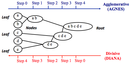
Hierarchical clustering can be divided into two main types: agglomerative and divisive.
Note that agglomerative clustering is good at identifying small clusters. Divisive hierarchical clustering is good at identifying large clusters.
As we learned in the k-means tutorial, we measure the (dis)similarity of observations using distance measures (i.e. Euclidean distance, Manhattan distance, etc.) In R, the Euclidean distance is used by default to measure the dissimilarity between each pair of observations. As we already know, it’s easy to compute the dissimilarity measure between two pairs of observations with the get_dist function.
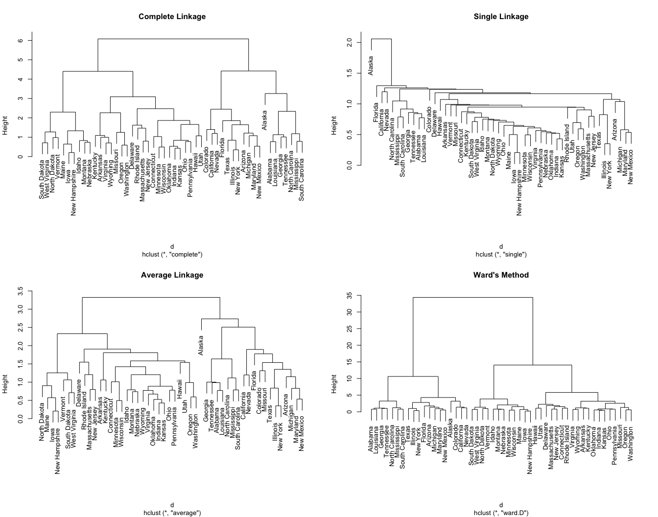
However, a bigger question is: How do we measure the dissimilarity between two clusters of observations? A number of different cluster agglomeration methods (i.e, linkage methods) have been developed to answer to this question. The most common types methods are:
We can see the differences these approaches in the following dendrograms:
To perform a cluster analysis in R, generally, the data should be prepared as follows:
Here, we’ll use the built-in R data set USArrests, which contains statistics in arrests per 100,000 residents for assault, murder, and rape in each of the 50 US states in 1973. It includes also the percent of the population living in urban areas
df <- USArrests
To remove any missing value that might be present in the data, type this:
df <- na.omit(df)
As we don’t want the clustering algorithm to depend to an arbitrary variable unit, we start by scaling/standardizing the data using the R function scale:
df <- scale(df)
head(df)
##                Murder   Assault   UrbanPop         Rape
## Alabama    1.24256408 0.7828393 -0.5209066 -0.003416473
## Alaska     0.50786248 1.1068225 -1.2117642  2.484202941
## Arizona    0.07163341 1.4788032  0.9989801  1.042878388
## Arkansas   0.23234938 0.2308680 -1.0735927 -0.184916602
## California 0.27826823 1.2628144  1.7589234  2.067820292
## Colorado   0.02571456 0.3988593  0.8608085  1.864967207
There are different functions available in R for computing hierarchical clustering. The commonly used functions are:
hclust [in stats package] and agnes [in cluster package] for agglomerative hierarchical clustering (HC)diana [in cluster package] for divisive HCWe can perform agglomerative HC with hclust. First we compute the dissimilarity values with dist and then feed these values into hclust and specify the agglomeration method to be used (i.e. “complete”, “average”, “single”, “ward.D”). We can then plot the dendrogram.
# Dissimilarity matrix
d <- dist(df, method = "euclidean")
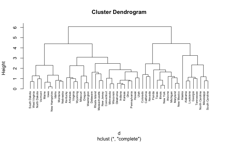
# Hierarchical clustering using Complete Linkage
hc1 <- hclust(d, method = "complete" )
# Plot the obtained dendrogram
plot(hc1, cex = 0.6, hang = -1)
Alternatively, we can use the agnes function. These functions behave very similarly; however, with the agnes function you can also get the agglomerative coefficient, which measures the amount of clustering structure found (values closer to 1 suggest strong clustering structure).
# Compute with agnes
hc2 <- agnes(df, method = "complete")

# Agglomerative coefficient
hc2$ac
## [1] 0.8531583
This allows us to find certain hierarchical clustering methods that can identify stronger clustering structures. Here we see that Ward’s method identifies the strongest clustering structure of the four methods assessed.
# methods to assess
m <- c( "average", "single", "complete", "ward")
names(m) <- c( "average", "single", "complete", "ward")

# function to compute coefficient
ac <- function(x) {
  agnes(df, method = x)$ac
}

map_dbl(m, ac)
##   average    single  complete      ward
## 0.7379371 0.6276128 0.8531583 0.9346210
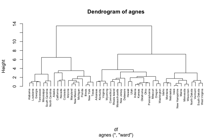
Similar to before we can visualize the dendrogram:
hc3 <- agnes(df, method = "ward")
pltree(hc3, cex = 0.6, hang = -1, main = "Dendrogram of agnes")
The R function diana provided by the cluster package allows us to perform divisive hierarchical clustering. diana works similar to agnes; however, there is no method to provide.
# compute divisive hierarchical clustering
hc4 <- diana(df)

# Divise coefficient; amount of clustering structure found
hc4$dc
## [1] 0.8514345

# plot dendrogram
pltree(hc4, cex = 0.6, hang = -1, main = "Dendrogram of diana")
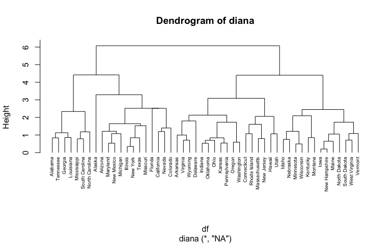
In the dendrogram displayed above, each leaf corresponds to one observation. As we move up the tree, observations that are similar to each other are combined into branches, which are themselves fused at a higher height.
The height of the fusion, provided on the vertical axis, indicates the (dis)similarity between two observations. The higher the height of the fusion, the less similar the observations are. Note that, conclusions about the proximity of two observations can be drawn only based on the height where branches containing those two observations first are fused. We cannot use the proximity of two observations along the horizontal axis as a criteria of their similarity.
The height of the cut to the dendrogram controls the number of clusters obtained. It plays the same role as the k in k-means clustering. In order to identify sub-groups (i.e. clusters), we can cut the dendrogram with cutree:
# Ward's method
hc5 <- hclust(d, method = "ward.D2" )

# Cut tree into 4 groups
sub_grp <- cutree(hc5, k = 4)

# Number of members in each cluster
table(sub_grp)
## sub_grp
##  1  2  3  4
##  7 12 19 12
We can also use the cutree output to add the the cluster each observation belongs to to our original data.
USArrests %>%
  mutate(cluster = sub_grp) %>%
  head
##   Murder Assault UrbanPop Rape cluster
## 1   13.2     236       58 21.2       1
## 2   10.0     263       48 44.5       2
## 3    8.1     294       80 31.0       2
## 4    8.8     190       50 19.5       3
## 5    9.0     276       91 40.6       2
## 6    7.9     204       78 38.7       2
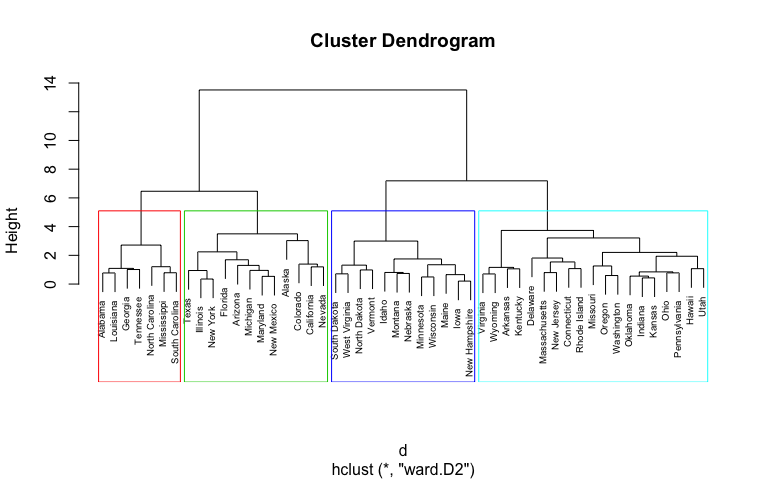
It’s also possible to draw the dendrogram with a border around the 4 clusters. The argument border is used to specify the border colors for the rectangles:
plot(hc5, cex = 0.6)
rect.hclust(hc5, k = 4, border = 2:5)
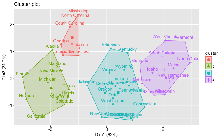
As we saw in the k-means tutorial, we can also use the fviz_cluster function from the factoextra package to visualize the result in a scatter plot.
fviz_cluster(list(data = df, cluster = sub_grp))
To use cutree with agnes and diana you can perform the following:
# Cut agnes() tree into 4 groups
hc_a <- agnes(df, method = "ward")
cutree(as.hclust(hc_a), k = 4)

# Cut diana() tree into 4 groups
hc_d <- diana(df)
cutree(as.hclust(hc_d), k = 4)
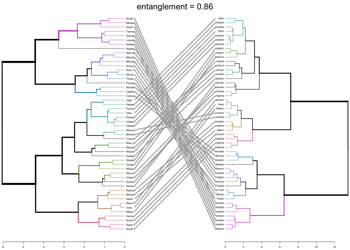
Lastly, we can also compare two dendrograms. Here we compare hierarchical clustering with complete linkage versus Ward’s method. The function tanglegram plots two dendrograms, side by side, with their labels connected by lines.
# Compute distance matrix
res.dist <- dist(df, method = "euclidean")

# Compute 2 hierarchical clusterings
hc1 <- hclust(res.dist, method = "complete")
hc2 <- hclust(res.dist, method = "ward.D2")

# Create two dendrograms
dend1 <- as.dendrogram (hc1)
dend2 <- as.dendrogram (hc2)

tanglegram(dend1, dend2)
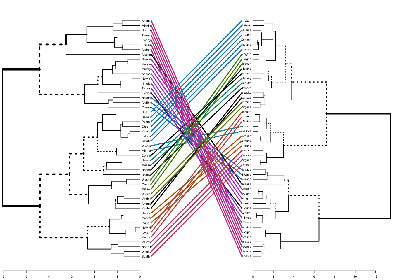
The output displays “unique” nodes, with a combination of labels/items not present in the other tree, highlighted with dashed lines. The quality of the alignment of the two trees can be measured using the function entanglement. Entanglement is a measure between 1 (full entanglement) and 0 (no entanglement). A lower entanglement coefficient corresponds to a good alignment. The output of tanglegram can be customized using many other options as follow:
dend_list <- dendlist(dend1, dend2)

tanglegram(dend1, dend2,
  highlight_distinct_edges = FALSE, # Turn-off dashed lines
  common_subtrees_color_lines = FALSE, # Turn-off line colors
  common_subtrees_color_branches = TRUE, # Color common branches
  main = paste("entanglement =", round(entanglement(dend_list), 2))
  )
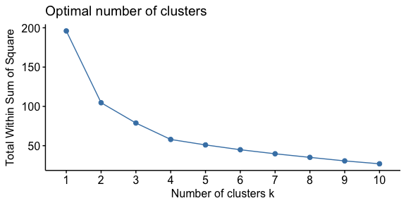
Similar to how we determined optimal clusters with k-means clustering, we can execute similar approaches for hierarchical clustering:
To perform the elbow method we just need to change the second argument in fviz_nbclust to FUN = hcut.
fviz_nbclust(df, FUN = hcut, method = "wss")
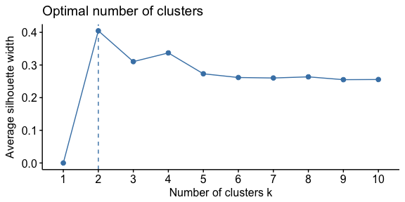
To perform the average silhouette method we follow a similar process.
fviz_nbclust(df, FUN = hcut, method = "silhouette")
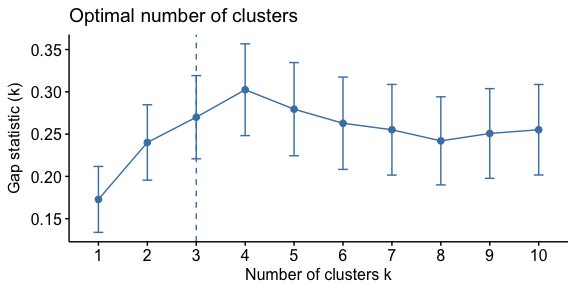
And the process is quite similar to perform the gap statistic method.
gap_stat <- clusGap(df, FUN = hcut, nstart = 25, K.max = 10, B = 50)
fviz_gap_stat(gap_stat)
Clustering can be a very useful tool for data analysis in the unsupervised setting. However, there are a number of issues that arise in performing clustering. In the case of hierarchical clustering, we need to be concerned about:
Each of these decisions can have a strong impact on the results obtained. In practice, we try several different choices, and look for the one with the most useful or interpretable solution. With these methods, there is no single right answer - any solution that exposes some interesting aspects of the data should be considered.
So, keep in mind that although hierarchical clustering can be performed quickly in R, there are many important variables to consider. However, this tutorial gets you started performing the hierarchical clustering approach and you can learn more with: