
It is often the case that some or many of the variables used in a multiple regression model are in fact not associated with the response variable. Including such irrelevant variables leads to unnecessary complexity in the resulting model. Unfortunately, manually filtering through and comparing regression models can be tedious. Luckily, several approaches exist for automatically performing feature selection or variable selection — that is, for identifying those variables that result in superior regression results. This tutorial will cover a traditional approach known as model selection.
This tutorial serves as an introduction to linear model selection and covers1:
This tutorial primarily leverages the Hitters data provided by the ISLR package. This is a data set that contains number of hits, homeruns, RBIs, and other information for 322 major league baseball players. We’ll also use tidyverse for some basic data manipulation and visualization. Most importantly, we’ll use the leaps package to illustrate subset selection methods.
# Packages
library(tidyverse)  # data manipulation and visualization
library(leaps)      # model selection functions

# Load data and remove rows with missing data
(
  hitters <- na.omit(ISLR::Hitters) %>%
    as_tibble
  )
## # A tibble: 263 × 20
##    AtBat  Hits HmRun  Runs   RBI Walks Years CAtBat CHits CHmRun CRuns
## *  <int> <int> <int> <int> <int> <int> <int>  <int> <int>  <int> <int>
## 1    315    81     7    24    38    39    14   3449   835     69   321
## 2    479   130    18    66    72    76     3   1624   457     63   224
## 3    496   141    20    65    78    37    11   5628  1575    225   828
## 4    321    87    10    39    42    30     2    396   101     12    48
## 5    594   169     4    74    51    35    11   4408  1133     19   501
## 6    185    37     1    23     8    21     2    214    42      1    30
## 7    298    73     0    24    24     7     3    509   108      0    41
## 8    323    81     6    26    32     8     2    341    86      6    32
## 9    401    92    17    49    66    65    13   5206  1332    253   784
## 10   574   159    21   107    75    59    10   4631  1300     90   702
## # ... with 253 more rows, and 9 more variables: CRBI <int>, CWalks <int>,
## #   League <fctr>, Division <fctr>, PutOuts <int>, Assists <int>,
## #   Errors <int>, Salary <dbl>, NewLeague <fctr>
To perform best subset selection, we fit a separate least squares regression for each possible combination of the p predictors. That is, we fit all p models that contain exactly one predictor, all models that contain exactly two predictors, and so forth. We then look at all of the resulting models, with the goal of identifying the one that is best.
The three-stage process of performing best subset selection includes:
Step 1: Let denote the null model, which contains no predictors. This model simply predicts the sample mean for each observation.
Step 2: For :
Step 3: Select a single best model from among using cross-validated prediction error, , AIC, BIC, or adjusted .
Let’s illustrate with our data. We can perform a best subset search using regsubsets (part of the leaps library), which identifies the best model for a given number of k predictors, where best is quantified using RSS. The syntax is the same as the lm function. By default, regsubsets only reports results up to the best eight-variable model. But the nvmax option can be used in order to return as many variables as are desired. Here we fit up to a 19-variable model.
best_subset <- regsubsets(Salary ~ ., hitters, nvmax = 19)
The resubsets function returns a list-object with lots of information. Initially, we can use the summary command to assess the best set of variables for each model size. So, for a model with 1 variable we see that CRBI has an asterisk signalling that a regression model with Salary ~ CRBI is the best single variable model. The best 2 variable model is Salary ~ CRBI + Hits. The best 3 variable model is Salary ~ CRBI + Hits + PutOuts. An so forth.
summary(best_subset)
## Subset selection object
## Call: regsubsets.formula(Salary ~ ., hitters, nvmax = 19)
## 19 Variables  (and intercept)
...
...
## 1 subsets of each size up to 19
## Selection Algorithm: exhaustive
##           AtBat Hits HmRun Runs RBI Walks Years CAtBat CHits CHmRun CRuns CRBI CWalks LeagueN DivisionW PutOuts Assists Errors NewLeagueN
## 1  ( 1 )  " "   " "  " "   " "  " " " "   " "   " "    " "   " "    " "   "*"  " "    " "     " "       " "     " "     " "    " "
## 2  ( 1 )  " "   "*"  " "   " "  " " " "   " "   " "    " "   " "    " "   "*"  " "    " "     " "       " "     " "     " "    " "
## 3  ( 1 )  " "   "*"  " "   " "  " " " "   " "   " "    " "   " "    " "   "*"  " "    " "     " "       "*"     " "     " "    " "
## 4  ( 1 )  " "   "*"  " "   " "  " " " "   " "   " "    " "   " "    " "   "*"  " "    " "     "*"       "*"     " "     " "    " "
## 5  ( 1 )  "*"   "*"  " "   " "  " " " "   " "   " "    " "   " "    " "   "*"  " "    " "     "*"       "*"     " "     " "    " "
## 6  ( 1 )  "*"   "*"  " "   " "  " " "*"   " "   " "    " "   " "    " "   "*"  " "    " "     "*"       "*"     " "     " "    " "
## 7  ( 1 )  " "   "*"  " "   " "  " " "*"   " "   "*"    "*"   "*"    " "   " "  " "    " "     "*"       "*"     " "     " "    " "
## 8  ( 1 )  "*"   "*"  " "   " "  " " "*"   " "   " "    " "   "*"    "*"   " "  "*"    " "     "*"       "*"     " "     " "    " "
## 9  ( 1 )  "*"   "*"  " "   " "  " " "*"   " "   "*"    " "   " "    "*"   "*"  "*"    " "     "*"       "*"     " "     " "    " "
## 10  ( 1 ) "*"   "*"  " "   " "  " " "*"   " "   "*"    " "   " "    "*"   "*"  "*"    " "     "*"       "*"     "*"     " "    " "
## 11  ( 1 ) "*"   "*"  " "   " "  " " "*"   " "   "*"    " "   " "    "*"   "*"  "*"    "*"     "*"       "*"     "*"     " "    " "
## 12  ( 1 ) "*"   "*"  " "   "*"  " " "*"   " "   "*"    " "   " "    "*"   "*"  "*"    "*"     "*"       "*"     "*"     " "    " "
## 13  ( 1 ) "*"   "*"  " "   "*"  " " "*"   " "   "*"    " "   " "    "*"   "*"  "*"    "*"     "*"       "*"     "*"     "*"    " "
## 14  ( 1 ) "*"   "*"  "*"   "*"  " " "*"   " "   "*"    " "   " "    "*"   "*"  "*"    "*"     "*"       "*"     "*"     "*"    " "
## 15  ( 1 ) "*"   "*"  "*"   "*"  " " "*"   " "   "*"    "*"   " "    "*"   "*"  "*"    "*"     "*"       "*"     "*"     "*"    " "
## 16  ( 1 ) "*"   "*"  "*"   "*"  "*" "*"   " "   "*"    "*"   " "    "*"   "*"  "*"    "*"     "*"       "*"     "*"     "*"    " "
## 17  ( 1 ) "*"   "*"  "*"   "*"  "*" "*"   " "   "*"    "*"   " "    "*"   "*"  "*"    "*"     "*"       "*"     "*"     "*"    "*"
## 18  ( 1 ) "*"   "*"  "*"   "*"  "*" "*"   "*"   "*"    "*"   " "    "*"   "*"  "*"    "*"     "*"       "*"     "*"     "*"    "*"
## 19  ( 1 ) "*"   "*"  "*"   "*"  "*" "*"   "*"   "*"    "*"   "*"    "*"   "*"  "*"    "*"     "*"       "*"     "*"     "*"    "*"
We can also get get the RSS, , adjusted , , and BIC from the results which helps us to assess the best overall model; however, we’ll illustrate this in the comparing models section. First, let’s look at how to perform stepwise selection.
For computational reasons, best subset selection cannot be applied when the number of p predictor variables is large. Best subset selection may also suffer from statistical problems when p is large. The larger the search space, the higher the chance of finding models that look good on the training data, even though they might not have any predictive power on future data. Thus an enormous search space can lead to overfitting and high variance of the coefficient estimates. For both of these reasons, stepwise methods, which explore a far more restricted set of models, are attractive alternatives to best subset selection.
Forward stepwise selection begins with a model containing no predictors, and then adds predictors to the model, one-at-a-time, until all of the predictors are in the model. In particular, at each step the variable that gives the greatest additional improvement to the fit is added to the model.
The three-stage process of performing forward stepwise selection includes:
Step 1: Let denote the null model, which contains no predictors. This model simply predicts the sample mean for each observation.
Step 2: For :
Step 3: Select a single best model from among using cross-validated prediction error, , AIC, BIC, or adjusted .
We can perform forward stepwise using regsubsets by setting method = "forward":
forward <- regsubsets(Salary ~ ., hitters, nvmax = 19, method = "forward")
Backward stepwise selection provides an efficient alternative to best subset selection. However, unlike forward stepwise selection, it begins with the full least squares model containing all p predictors, and then iteratively removes the least useful predictor, one-at-a-time.
The three-stage process of performing forward stepwise selection includes:
Step 1: Let denote the full model, which contains all p predictors.
Step 2: For :
Step 3: Select a single best model from among using cross-validated prediction error, , AIC, BIC, or adjusted .
We can perform backward stepwise using regsubsets by setting method = "backward":
backward <- regsubsets(Salary ~ ., hitters, nvmax = 19, method = "backward")
So far, I’ve illustrated how to perform the best subset and stepwise procedures. Now let’s discuss how to compare all the models that these approaches output in order to identify the best model. That is, let’s perform step 3 discussed in each of the 3-stage processes outlined above.
In order to select the best model with respect to test error, we need to estimate this test error. There are two common approaches:
We consider both of these approaches below.
When performing the best subset or stepwise approaches, the models selected are selected based on the fact that they minimize the training set mean square error (MSE).2 Because of this and the fact that using the training MSE and will bias our results we should not use these statistics to determine which of the models is “the best”.
However, a number of techniques for adjusting the training error for the model size are available. These approaches can be used to select among a set of models with different numbers of variables. These include:
| Statistic | Objective | Equation |
|---|---|---|
| Minimize | ||
| Akaike information criterion (AIC) | Minimize | |
| Bayesian information criterion (BIC) | Minimize | |
| adjusted | Maximize |
where d is the number of predictors and is an estimate of the variance of the error () associated with each response measurement in a regression model. Each of these statistics adds a penalty to the training RSS in order to adjust for the fact that the training error tends to underestimate the test error. Clearly, the penalty increases as the number of predictors in the model increases.
Therefore, these statistics provide an unbiased estimate of test MSE. If we perform our model using a training vs. testing validation approach we can use these statistics to determine the preferred model. These statistics are contained in the output provided by the regsubsets function. Let’s extract this information and plot them.
# create training - testing data
set.seed(1)
sample <- sample(c(TRUE, FALSE), nrow(hitters), replace = T, prob = c(0.6,0.4))
train <- hitters[sample, ]
test <- hitters[!sample, ]
# perform best subset selection
best_subset <- regsubsets(Salary ~ ., train, nvmax = 19)
results <- summary(best_subset)
# extract and plot results
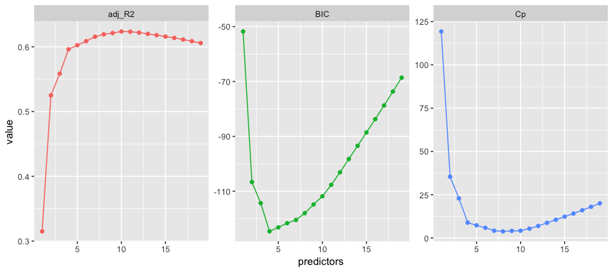
tibble(predictors = 1:19,
adj_R2 = results$adjr2,
Cp = results$cp,
BIC = results$bic) %>%
gather(statistic, value, -predictors) %>%
ggplot(aes(predictors, value, color = statistic)) +
geom_line(show.legend = F) +
geom_point(show.legend = F) +
facet_wrap(~ statistic, scales = "free")
Here we see that our results identify slightly different models that are considered the best. The adjusted statistic suggests the 10 variable model is preferred, the BIC statistic suggests the 4 variable model, and the suggests the 8 variable model.3
which.max(results$adjr2)
## [1] 10
which.min(results$bic)
## [1] 4
which.min(results$cp)
## [1] 8
We can compare the variables and coefficients that these models include using the coef function.
# 10 variable model
coef(best_subset, 10)
## (Intercept)       AtBat        Hits       Walks      CAtBat       CHits
## -47.3715661  -1.3695666   6.3013473   4.5757613  -0.3118794   1.4799307
##      CHmRun      CWalks     LeagueN   DivisionW     PutOuts
##   1.2971405  -0.5026157  62.5613310 -62.3548737   0.2527181

# 4 variable model
coef(best_subset, 4)
## (Intercept)        Runs      CAtBat       CHits     PutOuts
## -83.1199265   5.5530883  -0.4741822   2.0560595   0.3118252

# 8 variable model
coef(best_subset, 8)
## (Intercept)       AtBat        Hits       Walks      CAtBat       CHits
## -59.2371674  -1.4744877   6.6802515   4.4777879  -0.3203862   1.5160882
##      CHmRun      CWalks     PutOuts
##   1.1861142  -0.4714870   0.2748103
We could perform the same process using forward and backward stepwise selection and obtain even more options for optimal models. For example, if I assess the optimal for forward and backward stepwise we see that they suggest that an 8 variable model minimizes the statistic, similar to the best subset approach above.
forward <- regsubsets(Salary ~ ., train, nvmax = 19, method = "forward")
backward <- regsubsets(Salary ~ ., train, nvmax = 19, method = "backward")

# which models minimize Cp?
which.min(summary(forward)$cp)
## [1] 8
which.min(summary(backward)$cp)
## [1] 8
However, when we assess these models we see that the 8 variable models include different predictors. Although, all models include AtBat, Hits, Walks, CWalks, and PutOuts, there are unique variables in each model.
coef(best_subset, 8)
## (Intercept)       AtBat        Hits       Walks      CAtBat       CHits
## -59.2371674  -1.4744877   6.6802515   4.4777879  -0.3203862   1.5160882
##      CHmRun      CWalks     PutOuts
##   1.1861142  -0.4714870   0.2748103
coef(forward, 8)
##  (Intercept)        AtBat         Hits        Walks        CRuns
## -112.7724200   -2.1421859    8.8914064    5.4283843    0.8555089
##         CRBI       CWalks      LeagueN      PutOuts
##    0.4866528   -0.9672115   64.1628445    0.2767328
coef(backward, 8)
## (Intercept)       AtBat        Hits       Walks      CAtBat       CHits
## -59.2371674  -1.4744877   6.6802515   4.4777879  -0.3203862   1.5160882
##      CHmRun      CWalks     PutOuts
##   1.1861142  -0.4714870   0.2748103
This highlights two important findings:
This is why it is important to always perform validation; that is, to always estimate the test error directly either by using a validation set or using cross-validation.
We now compute the validation set error for the best model of each model size. We first make a model matrix from the test data. The model.matrix function is used in many regression packages for build- ing an “X” matrix from data.
test_m <- model.matrix(Salary ~ ., data = test)
Now we can loop through each model size (i.e. 1 variable, 2 variables,…, 19 variables) and extract the coefficients for the best model of that size, multiply them into the appropriate columns of the test model matrix to form the predictions, and compute the test MSE.
# create empty vector to fill with error values
validation_errors <- vector("double", length = 19)

for(i in 1:19) {
  coef_x <- coef(best_subset, id = i)                     # extract coefficients for model size i
  pred_x <- test_m[ , names(coef_x)] %*% coef_x           # predict salary using matrix algebra
  validation_errors[i] <- mean((test$Salary - pred_x)^2)  # compute test error btwn actual & predicted salary
}

# plot validation errors
plot(validation_errors, type = "b")
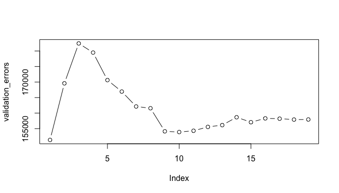
Here, we actually see that the 1 variable model produced by the best subset approach produces the lowest test MSE! If we repeat this using a different random value seed, we will get a slightly different model that is the “best”. However, if you recall from the Resampling Methods tutorial, this is to be expected when using a training vs. testing validation approach.
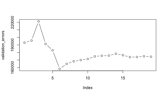
# create training - testing data
set.seed(5)
sample <- sample(c(TRUE, FALSE), nrow(hitters), replace = T, prob = c(0.6,0.4))
train <- hitters[sample, ]
test <- hitters[!sample, ]

# perform best subset selection
best_subset <- regsubsets(Salary ~ ., train, nvmax = 19)

# compute test validation errors
test_m <- model.matrix(Salary ~ ., data = test)
validation_errors <- vector("double", length = 19)

for(i in 1:19) {
  coef_x <- coef(best_subset, id = i)                     # extract coefficients for model size i
  pred_x <- test_m[ , names(coef_x)] %*% coef_x           # predict salary using matrix algebra
  validation_errors[i] <- mean((test$Salary - pred_x)^2)  # compute test error btwn actual & predicted salary
}

# plot validation errors
plot(validation_errors, type = "b")
A more robust approach is to perform cross validation. But before we do, let’s turn our our approach above for computing test errors into a function. Our function pretty much mimics what we did above. The only complex part is how we extracted the formula used in the call to regsubsets. I suggest you work through this line-by-line to understand what each step is doing.
predict.regsubsets <- function(object, newdata, id ,...) {
  form <- as.formula(object$call[[2]])
  mat <- model.matrix(form, newdata)
  coefi <- coef(object, id = id)
  xvars <- names(coefi)
  mat[, xvars] %*% coefi
  }
We now try to choose among the models of different sizes using k-fold cross-validation. This approach is somewhat involved, as we must perform best subset selection within each of the k training sets. First, we create a vector that allocates each observation to one of k = 10 folds, and we create a matrix in which we will store the results.
k <- 10
set.seed(1)
folds <- sample(1:k, nrow(hitters), replace = TRUE)
cv_errors <- matrix(NA, k, 19, dimnames = list(NULL, paste(1:19)))
Now we write a for loop that performs cross-validation. In the jth fold, the elements of folds that equal j are in the test set, and the remainder are in the training set. We make our predictions for each model size, compute the test errors on the appropriate subset, and store them in the appropriate slot in the matrix cv_errors.
for(j in 1:k) {

  # perform best subset on rows not equal to j
  best_subset <- regsubsets(Salary ~ ., hitters[folds != j, ], nvmax = 19)

  # perform cross-validation
  for( i in 1:19) {
    pred_x <- predict.regsubsets(best_subset, hitters[folds == j, ], id = i)
    cv_errors[j, i] <- mean((hitters$Salary[folds == j] - pred_x)^2)
    }
  }
This has given us a 10×19 matrix, of which the (i,j)th element corresponds to the test MSE for the ith cross-validation fold for the best j-variable model. We use the colMeans function to average over the columns of this matrix in order to obtain a vector for which the jth element is the cross-validation error for the j-variable model.
mean_cv_errors <- colMeans(cv_errors)

plot(mean_cv_errors, type = "b")
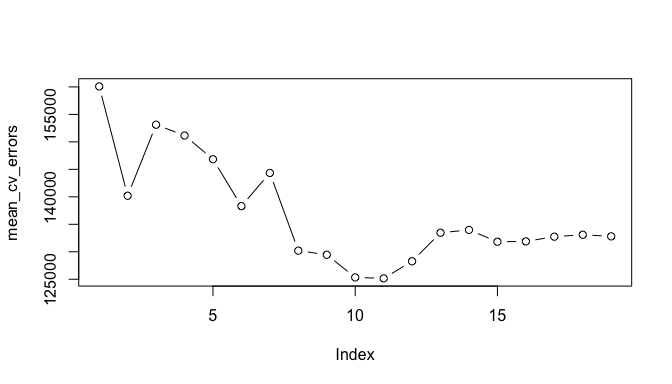
We see that our more robust cross-validation approach selects an 11-variable model. We can now perform best subset selection on the full data set in order to obtain the 11-variable model.
final_best <- regsubsets(Salary ~ ., data = hitters , nvmax = 19)
coef(final_best, 11)
##  (Intercept)        AtBat         Hits        Walks       CAtBat
##  135.7512195   -2.1277482    6.9236994    5.6202755   -0.1389914
##        CRuns         CRBI       CWalks      LeagueN    DivisionW
##    1.4553310    0.7852528   -0.8228559   43.1116152 -111.1460252
##      PutOuts      Assists
##    0.2894087    0.2688277
This will get you started with approaches for performing linear model selection; however, understand that there are other approaches for more sophisticated model selection procedures. The following resources will help you learn more:
This tutorial was built as a supplement to section 6.1 of An Introduction to Statistical Learning. ↩
Technically, it minimizes the RSS but recall that $MSE = RSS/n$ so MSE is minimized by association. ↩
These statistics differ for important reasons. Furthermore, some of these statistics are motivated more by statistical theory than others. For more information behind these statistics I would suggest starting by reading section 6.1 of An Introduction to Statistical Learning. ↩