
The relatively recent explosion in available computing power allows for old methods to be reborn as well as new methods to be created. One such machine learning algorithm that is directly the product of the computer age is the random forest, a computationally extensive prediction algorithm based on bootstrapped decision trees which possesses impressive predictive capability. Another machine learning algorithm, known as boosting, has taken prediction accuracy a step further, using sequential decision trees to fine-tune the analysis.
We will leverage several packages that the user will need to install prior to working through the tutorial. ISLR contains the Hitters data set that is used to demonstrate tree-based regression methods. The other four packages listed, rpart, rpart.plot, randomForest, and gbm, contain functions that support the methodology and visualization capability required for decision trees, random forests, and boosting. Also, the Heart data set is read into R from the url listed below, and will be used to demonstrate tree-based classification.
# attach necessary packages
library(ISLR)           # data sets
library(rpart)          # decision tree methodology
library(rpart.plot)     # decision tree visualization
library(randomForest)   # random forest methodology
library(gbm)            # boosting methodology
# read in Heart data set
Heart <- read.csv("http://www-bcf.usc.edu/~gareth/ISL/Heart.csv")
# ensure reproducibility
set.seed(200)
Before conducting any analysis, we transform the Salary variable in Hitters by taking the log. Without taking the log, salaries tend to be highly skewed. Tree-based methods are not typically robust to outliers, so this transformation will help eliminate them. We also split our data into training and testing sets, so that model validation may be performed later.
# transform salary variable to the logarithm of salary
Hitters$Salary <- log(Hitters$Salary)
# sample 70% of the row indices for training the models
trainHit <- sample(1:nrow(Hitters), 0.7*nrow(Hitters))
trainHeart <- sample(1:nrow(Heart), 0.7*nrow(Heart))
Hitters is a data set that contains 20 statistics on 322 players from the 1986 and 1987 seasons; we randomly select 70% of these observations (225 players) for our training set, leaving 30% (97 players) for validation. The Heart data set contains 14 heart health-related characteristics on 303 patients. We will also use a 70/30 split for training and testing, with 212 patients making up the training set and 91 patients left for validation. Random forests and boosting are both best suited for large data sets, but these data sets will function as good examples for the purpose of this tutorial.
Random Forests and Boosting are techniques derived from the decision tree, which segments the feature space of a data set by minimizing the total variance at each step. Decision trees are conceptually straightforward and visually appealing, as a new observation need only follow the path specified by its predictors in order to reach the estimated value/class. In R, the rpart() command from the rpart package fits a simple decision tree. We will use the Hitters data set from the ISLR package and the prp plot command to demonstrate a regression tree that fits a continuous response: the log salary of each player based on number of years in the league and number of hits the previous season.
# fit decision tree to Hitters data
salfit <- rpart(formula = Salary ~ Years + Hits, data = Hitters[trainHit,],
                   method = "anova", control = rpart.control(maxdepth = 2))
# display results
prp(salfit)
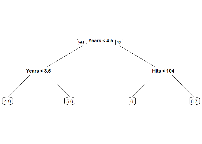
Note the ease of interpretation. If we want to predict the log salary of a new hitter who had been in the league for 5 seasons and had 110 hits the previous season, we would start at the top of the tree and compare 5 years to 4.5 years. Seeing that 5 is not less than 4.5, we choose the right branch. Reaching the next split, we see that 110 hits is greater than 104 and choose the right branch at this split, arriving at our log salary estimate of 6.7 for our new player (which corresponds to a salary point estimate of $812,405.80).
The additional arguments to rpart give the user some control over how the tree is fit. We specify in the first argument that we wish to predict Salary using Hits and Years as predictors, specifying in the second argument that these variables are to be taken from the training observations of Hitters. Because our response variable is continuous, we set method = "anova". Lastly, to fine-tune our analysis options, we specified that the tree should contain 2 levels of branches.
But if we want the best prediction, how could we know beforehand how many levels to include? By default, rpart will cross-validate the results of the tree and trim the tree (this is called pruning). We re-fit the model without controlling the depth and examine the results, this time using a command from rpart.plot to visualize the tree:
# fit decision tree without controlling depth
salfit <- rpart(formula = Salary ~ Years + Hits, data = Hitters[trainHit,], method = "anova")
# display results
rpart.plot(salfit)
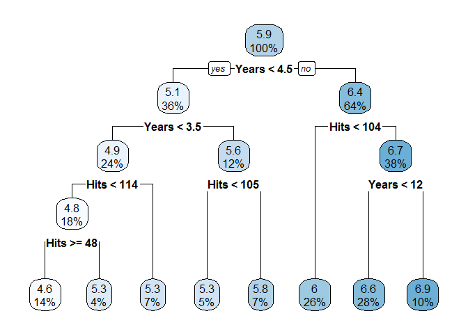
Based on this new, cross-validated decision tree, the estimate for the log salary of our new hitter becomes 6.6 ($735,095.20), and we can reasonably expect to have slightly more confidence in the accuracy of this point estimate. Each node in this visual display gives the estimate at each node as well as the percentage of training observations that are placed in that node. We can use the predict function to estimate the log salary for every hitter in the testing set as well as calculate the total error.
# predict testing set - show first four predictions
predict(salfit, Hitters[-trainHit,])[1:4]
##      -Alvin Davis        -Al Newman       -Bill Almon -Buddy Biancalana
##          5.280013          5.265399          6.003444          6.003444
# calculate SSE
(treeSSE <- sum((predict(salfit, Hitters[-trainHit,]) - Hitters$Salary[-trainHit])^2, na.rm = TRUE))
## [1] 22.00845
To measure the performance of a decision tree for regression, the sum of squared errors (SSE) is calculated for the observations in the testing set. This decision tree gives a sum of squared errors of 22.008, which will provide a baseline to compare the more advanced methods to.
Decision trees are not limited to continuous response variables, however. As an example of a classification problem, we turn to the Heart data set. We attempt to predict whether a patient has heart disease (AHD) based on some health-related characteristics. Before fitting the model, we take the row identifier (X) out of the data frame. It wouldn’t make sense for an identification number to have predictive ability, so we assume that if it were included, it could only be marked as significant by random chance.
# Take out the row identifier as a predictor
Heart <- Heart[,-which(colnames(Heart) == "X")]
# fit classification decision tree
AHDfit <- rpart(AHD ~ ., data = Heart[trainHeart,], method = "class")
# display results
rpart.plot(AHDfit)
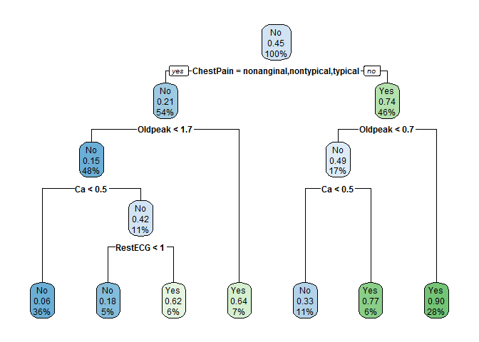
We see that the first split is on the ChestPain variable, which is categorical. For categorical variables, the splits are done by factor level, where the “nonanginal”, “nontypical”, and “typical” categories correspond to the left path and all other levels correspond to the right path. In our case, the right path represents the “asymptomatic” condition. At subsequent splits, the other variables needed to determine the estimate are Oldpeak, Ca, and RestECG.
# predict the patients in the testing set
predict(AHDfit, Heart[-trainHeart,])[1:4]
## [1] 0.1000000 0.3571429 0.1000000 0.6666667
You may have noticed that this decision tree includes an additional piece of information: the node purity. If 100% of the observations in a given node were “Yes”, the box would be dark green and the node purity would be 100%. This concept will be revisited later in the tutorial to estimate variable importance. This also allows us to quantify how likely a new patient is to be in each category, instead of just a point estimate. For example, the first patient in the testing set is classified as “No”, but is further clarified to have a 10% chance of being “Yes”.
# confusion matrix
(treeT <- table(predict(AHDfit, Heart[-trainHeart,], type = "class"),Heart$AHD[-trainHeart]))
##
##       No Yes
##   No  30   8
##   Yes 18  35
The classification accuracy of the tree is 71.4%, which is better than just assigning observations randomly with equal probability, but not as high as we would like given the amount of pertinent information we believe we possess.
Decision trees are easy to interpret, but tend to perform relatively poorly in prediction. The estimates themselves are unbiased, but the large variability associated with trees tends to make for large confidence bounds and inaccurate predictions. In order to increase the predictive accuracy of the method, we need to grow more trees.
Each tree grown has low bias and high variability, so in order to decrease the variability, we can calculate the average estimate over a large number of trees. By bootstrapping the data, we can generate a large number of trees and then average the prediction (for regression problems) or take a vote (for classification problems). This technique is called bagging, and can be performed with the randomForest command from the randomForest package by setting the mtry argument equal to the number of predictors.
# fit bagging model
bag_salary <- randomForest(Salary ~ ., data = Hitters[trainHit,], mtry = (ncol(Hitters)-1), ntree = 5000)
When we attempt to fit this model, however, we receive an error. Bagging (and also random forests) cannot be performed with missing values in the predictors or response. These missing values cause issues with calculations used for determining splits. So in order to fit a bagging model, we use the complete.cases function to select only the 184 observations in the training set that have a complete set of variables. If there are missing values in the testing set, the predict function does not produce an error, but the prediction is marked as missing.
# get indices of complete cases
fullHit <- (1:nrow(Hitters))[complete.cases(Hitters)]
# fit bagging algorithm
bag_salary <- randomForest(Salary ~ ., data = Hitters[intersect(fullHit,trainHit),],
                       mtry = (ncol(Hitters)-1), ntree = 5000)
# predict new values
predict(bag_salary, Hitters[-trainHit,])[5:8]
##   -Bruce Bochy     -Bob Boone  -Brett Butler -Billy Hatcher
##       5.276285       6.720920       6.271461       4.771774
Using bagging, our point estimates may or may not be similar to the point estimates predicted by a single decision tree, but will always have smaller variance, and therefore better predictive performance on the whole. We can calculate the sum of squared errors the same way we did for trees:
# calculate sum of squared errors
(bagSSE <- sum((predict(bag_salary, Hitters[-trainHit,]) - Hitters$Salary[-trainHit])^2, na.rm = TRUE))
## [1] 12.50323
Our SSE of 12.503 is dramatically smaller than the single decision tree used earlier. We set the number of trees to be 5000, but this decision doesn’t need fine-tuning; as long as our number of trees is sufficiently large, the error will not be improved by increasing this value.
We can perform the same process for the classification example, using all predictor variables at each split and planting 5000 trees for analysis.
# get indices of complete cases
fullHeart <- (1:nrow(Heart))[complete.cases(Heart)]
# fit bagging algorithm
bag_heart <- randomForest(AHD ~ ., data = Heart[intersect(fullHeart,trainHeart),],
                         mtry = (ncol(Heart)-1), ntree = 5000)
# predict new values
predict(bag_heart,Heart[-trainHeart,])[5:8]
## 12 17 20 22
## No No No No
## Levels: No Yes
# confusion matrix
(bagT <- table(predict(bag_heart, Heart[-trainHeart,], type = "class"),Heart$AHD[-trainHeart]))
##
##       No Yes
##   No  39   6
##   Yes  7  37
Based on the confusion matrix, our classification accuracy for bagging is 85.4%, which outperforms the single tree used previously. Bagging estimates retain the unbiased property that makes decision trees desirable while decreasing the variance, but we can do even better. A simple tweak in the process can decrease the variance of our estimates even further. Bagging is infrequently used in practice, due to the efficiency of random forests, its conceptual cousin.
Random Forests are similar to bagging, except that instead of choosing from all variables at each split, the algorithm chooses from a random subset. This subtle tweak decorrelates the trees, which reduces the variance of the estimates while maintaining the unbiasedness of the point estimate. We again use the randomForest function to fit a random forest model to the Hitters data. To combat missingness, we could choose to impute the missing values by changing the na.action argument.
# impute missing values instead of causing an issue
rf_salary <- randomForest(Salary ~ ., data = Hitters[trainHit,], na.action = na.roughfix)
Instead of sticking with the imputed data, we keep only the full cases. By default, the randomForest function uses the square root of the number of predictors at each split, which is a good rule-of-thumb to produce good results in practice. By adding the importance argument, we can later examine relative importance scores for the variables.
# fit random forest algorithm
rf_salary <- randomForest(Salary ~ ., data = Hitters[intersect(fullHit, trainHit),],
                          ntree = 5000, importance = TRUE)
# make predictions
predict(rf_salary, Hitters[-trainHit,])[9:12]
##      -Bob Kearney    -Butch Wynegar -Carmelo Martinez    -Charlie Moore
##          5.706444          6.079991          5.796563          5.965687
# calculate sum of squared errors
(rfSSE <- sum((predict(rf_salary, Hitters[-trainHit,]) - Hitters$Salary[-trainHit])^2, na.rm = TRUE))
## [1] 11.56442
The sum of squared errors using a random forest approach is 11.564. This improves even upon the bagging figure, though the effect isn’t as great as the change from a single tree to bagging. Random forests build deep trees with many, many levels of splits. It learns quickly and then averages or votes using the results. For classification using random forests, the process is the same as before, where we can predict the category of each test set observation.
# fit random forest algorithm
rf_heart <- randomForest(AHD ~ ., data = Heart[intersect(fullHeart, trainHeart),], ntree = 5000)
# make predictions
predict(rf_heart, Heart[-trainHeart,])[9:12]
##  24  25  27  29
## Yes Yes  No  No
## Levels: No Yes
# confusion matrix
(rfT <- table(predict(rf_heart, Heart[-trainHeart,], type = "class"), Heart$AHD[-trainHeart]))
##
##       No Yes
##   No  41   6
##   Yes  5  37
The classification accuracy rate is also improved from bagging, with a rate of 87.6%.
When fitting random forests (as well as in bagging), not every training set observation is used in each bootstrapped data set. In fact, normally, around 37% of observations are left out of each tree being fit. One method for measuring the error is called “out-of-bag” (OOB) error, where the model is fit to these observations that were not included in the bootstrap.
This OOB error measure can be used to verify that we have planted enough trees. Random forests do not begin to overfit as the number of trees increases; it just has to be verified that the error has stabilized. By using the plot command, we can plot OOB error as a function of the number of trees.
# plot OOB error as a function of number of trees
plot(rf_salary)
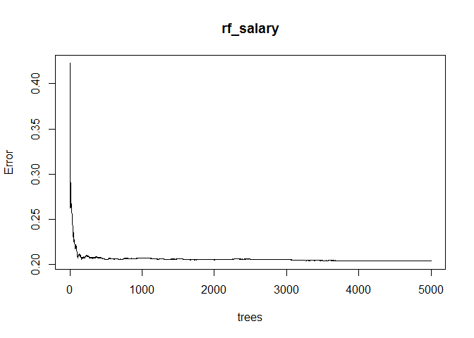
The plot indicates that 5000 trees is enough for the OOB error to have stabilized, so we can be confident that our random forest model is not suffering from underfitting.
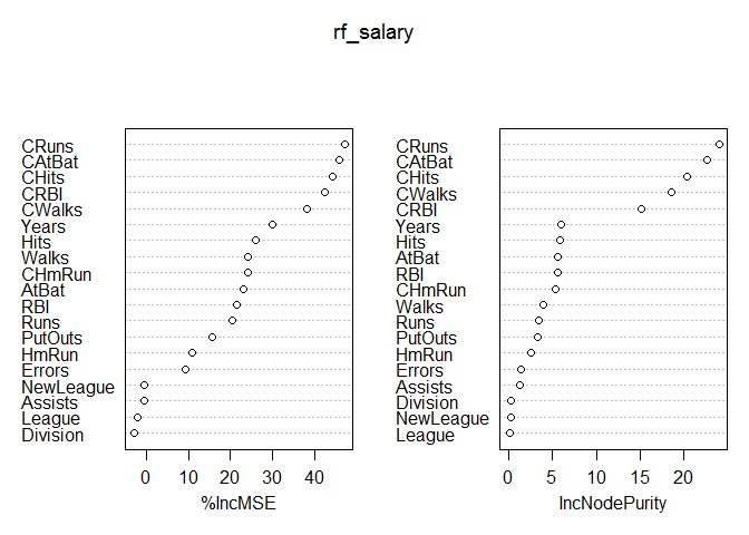
Once the predictions have been made, a natural follow-up question to ask is which variables were the most important in calculating the estimates. In order to examine variable importance for each predictor variable, we can call the importance function:
# list relative measure of variable importance
importance(rf_salary)
##              %IncMSE IncNodePurity
## AtBat     22.9793810     5.6464281
## Hits      26.0049181     5.8538937
## HmRun     10.9110307     2.5174891
## Runs      20.3043055     3.4717977
## RBI       21.5380047     5.5702355
## Walks     24.2257382     3.8990224
## Years     30.0031322     6.0506872
## CAtBat    45.9132544    22.6418724
## CHits     44.1987717    20.3973787
## CHmRun    24.0351669     5.3013462
## CRuns     47.0675346    24.0092790
## CRBI      42.4186220    15.1864142
## CWalks    38.1232239    18.5629225
## League    -2.0609131     0.1892874
## Division  -2.9306789     0.2224646
## PutOuts   15.5055641     3.3158257
## Assists   -0.5787550     1.2760977
## Errors     9.3546942     1.4284182
## NewLeague -0.4761242     0.2165269
Variable importance for random forests models is calculated using two different methods that generally produce similar results. The first method listed is percent increase in Mean Squared Error, while the second method is the increase in node purity. We can visualize these results using the varImpPlot function, which plots the variables using the same two methods.
# plot variable importance
varImpPlot(rf_salary)
Random forests purposefully overfit each bootstrapped data set and then compensate by averaging over a large number of trees. Another approach to training data is by planting purposefully underfitted trees that learn slowly and are built sequentially, also known as Boosting.
We can fit a boosted model using the gbm function from the gbm package. Boosting is far more customizable than random forests, but therefore requires more effort to properly tune. In addition to the n.tree argument present in random forests, the user can control a number of other hyperparameters, including the distribution of the residuals (distribution), how deep to plant each tree (interaction.depth), and how fast the model learns (shrinkage). In our first model, we also chose to use 5-fold cross-validation. When properly tuned, boosting can be expected to perform at or above the predictive level of random forests, with the added bonus of being able to handle missing values.
# fit boosting model
boost_salary <- gbm(Salary ~ ., data = Hitters[intersect(fullHit,trainHit),],
                 distribution = "gaussian", n.trees = 10000, interaction.depth = 4, cv.folds = 5)
Unlike random forests, overfitting is a serious concern as the number of trees increases for boosting, so we use the gbm.perf function to find the “best” value for the number of trees based on some measure of error (in our case, we use the cross-validation error).
# find the best number of trees using the cross-validation error
bestHit <- gbm.perf(boost_salary, method = "cv")
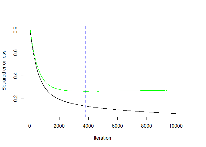
Once this sweet spot has been found, we can make predictions and calculate the sum of squared errors as before, taking note of the fact that predict requires the n.trees argument to be set.
# predict values
predict(boost_salary, Hitters[-trainHit,], n.trees = bestHit)[13:16]
## [1] 5.951279 6.873412 5.036994 5.656109
# calculate sum of squared errors
(boostSSE <- sum((predict(boost_salary, Hitters[-trainHit,], n.trees = bestHit) - Hitters$Salary[-trainHit])^2,
                 na.rm = TRUE))
## [1] 12.60176
The sum of squared errors on the testing set for the boosted model is 12.602, a number that is worse than both random forest and bagging. This can happen for a first model fit in boosting. In order to decrease the SSE, we try different values of the available hyperparameters, such as the interaction depth.
# testing the effect of interaction depth using a gaussian loss function
(IntDepthG <- sapply(1:8, function(x) {
  # fit model
  boost_salary <- gbm(Salary ~ .,
                   data = Hitters[intersect(fullHit,trainHit),],
                   distribution = "gaussian",
                   n.trees = 15000,
                   interaction.depth = x,
                   shrinkage = 0.001,
                   cv.folds = 5)
  # calculate best value for number of trees
  bestHit <- gbm.perf(boost_salary, method = "cv", plot.it = FALSE)
  # calculate the sum of squared errors
  boostSSE <- sum((predict(boost_salary, Hitters[-trainHit,], n.trees = bestHit) - Hitters$Salary[-trainHit])^2,
                 na.rm = TRUE)
  return(boostSSE)}))
## [1] 14.38035 13.16236 12.94303 13.29108 12.80670 12.68734 12.69801 13.16019
No matter the interaction depth, none of these models perform as well as the random forest model, so we can assume that the normal distribution does not fit the residuals well. We can try a different loss function and see how the interaction depth affects the error:
# testing the effect of interaction depth using a gaussian loss function
(IntDepthT <- sapply(1:8, function(x) {
  # fit model
  boost_salary <- gbm(Salary ~ .,
                   data = Hitters[intersect(fullHit,trainHit),],
                   distribution = "tdist",
                   n.trees = 15000,
                   interaction.depth = x,
                   shrinkage = 0.001,
                   cv.folds = 5)
  # calculate the best value for number of trees
  bestHit <- gbm.perf(boost_salary, method = "cv", plot.it = FALSE)
  # calculate the sum of squared errors
  boostSSE <- sum((predict(boost_salary,Hitters[-trainHit,], n.trees = bestHit) - Hitters$Salary[-trainHit])^2,
                 na.rm = TRUE)
  return(boostSSE)}))
## [1] 11.91072 11.01530 10.81030 10.74081 10.72682 10.70409 10.96769 11.21215
The heavy tailed t-distribution (with default 4 degrees of freedom) produces a far better fit, outperforming the random forest model for almost any interaction depth tested. To minimize SSE, we choose to fit a model with a t-distribution, interaction depth of 6, and shrinkage of 0.001. Our SSE in that instance is 10.704.
For classification problems, the response value must be converted to a 0/1 response in gbm. This model is fit with the distribution argument set to "bernoulli". Then the same procedure is followed.
# convert response to 0/1
Heart$AHD <- ifelse(Heart$AHD == "Yes",1,0)
# fit boosting model to Heart data
boost_heart <- gbm(AHD ~ ., data = Heart[intersect(fullHeart,trainHeart),],
                     distribution = "bernoulli", n.trees = 10000, shrinkage = 0.001,
                   interaction.depth = 3, cv.folds = 5)
bestHeart <- gbm.perf(boost_heart, method = "cv", plot.it = FALSE)
Just as with continuous response variables, we can try different values of the hyperparameters to see which values fit our data best.
# fit boosting model
(ClassRate <- sapply(1:8, function(x) {
  boost_heart <- gbm(AHD ~ ., data = Heart[intersect(fullHeart,trainHeart),],
                     distribution = "bernoulli", n.trees = 10000, shrinkage = 0.001,
                     interaction.depth = x, cv.folds = 5)
  # find best number of trees
  bestHeart <- gbm.perf(boost_heart, method = "cv", plot.it = FALSE)
  predHeart <- ifelse(predict(boost_heart, Heart[-trainHeart,], n.trees = bestHeart) > 0.5,"Yes","No")
  # calculate misclassification rate
  cr <- sum(diag(table(predHeart, Heart$AHD[-trainHeart]))) / sum(table(predHeart, Heart$AHD[-trainHeart]))
  return(cr)
}))
## [1] 0.8571429 0.8571429 0.8791209 0.8791209 0.8791209 0.8681319 0.8901099
## [8] 0.8791209
This process indicates that the optimal interaction depth for predicting AHD is 7, which produces a classification prediction rate of 89%, outperforming the random forest high mark. Once an acceptable model has been found, we can perform variable importance analysis:
# fit optimal model
boost_heart <- gbm(AHD ~ ., data = Heart[intersect(fullHeart, trainHeart),],
                   distribution = "bernoulli", n.trees = 10000, shrinkage = 0.001,
                   interaction.depth = which.max(ClassRate), cv.folds = 5)
bestHeart <- gbm.perf(boost_heart, method = "cv", plot.it = FALSE)
# plot variable importance
par(mar = c(5,5,4,2))
summary(boost_heart, n.trees = bestHeart, las = 1)
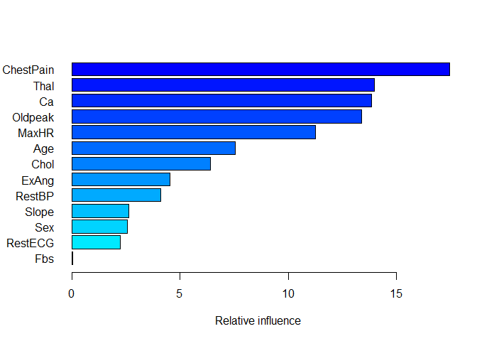
##                 var     rel.inf
## ChestPain ChestPain 17.46216698
## Thal           Thal 13.96502176
## Ca               Ca 13.83959162
## Oldpeak     Oldpeak 13.38918621
## MaxHR         MaxHR 11.26476204
## Age             Age  7.53929757
## Chol           Chol  6.41846002
## ExAng         ExAng  4.54440015
## RestBP       RestBP  4.10693112
## Slope         Slope  2.63133173
## Sex             Sex  2.56533294
## RestECG     RestECG  2.22506765
## Fbs             Fbs  0.04845022
The summary function shows the relative variable importance scores for the optimized boosting model, with ChestPain being the most important variable used to make predictions. Unsurprisingly, some of the same variables used in our initial decision tree turn out to be important in the boosting model, but we can now quantify how much so and order the variables by importance. We can fit our best model and verify the accuracy:
# confusion matrix
predHeart <- ifelse(predict(boost_heart, Heart[-trainHeart,], n.trees = bestHeart) > 0.5,"Yes","No")
(boostT <- table(predHeart, Heart$AHD[-trainHeart]))
##
## predHeart  0  1
##       No  45  7
##       Yes  3 36
The prediction accuracy of the boosted model is 89%. The boosting algorithm is applicable to many other methods besides tree-based methods, with the concept of fitting to residuals enabling the method to remain effective under almost any situation.