
 Resampling methods are an indispensable tool in modern statistics. They involve repeatedly drawing samples from a training set and recomputing an item of interest on each sample. Bootstrapping is one such resampling method that repeatedly draws independent samples from our data set and provides a direct computational way of assessing uncertainty. This tutorial covers the basics of bootstrapping to estimate the accuracy of a single statistic. Note that resampling (to include bootstrapping) to improve the bias-variance tradeoff in predictive modeling is discussed elsewhere.
First, I cover the packages and data used to reproduce results displayed in this tutorial. I then discuss how boostrapping works followed by illustrating how to implement the method in R.
This tutorial primarily uses the rsample package to create bootstrap samples but also uses the purrr and ggplot2 packages (both contained in tidyverse). To illustrate, our example attrition data comes from the rsample package.
library(tidyverse)
library(rsample)

as_tibble(attrition)
## # A tibble: 1,470 x 31
##      Age Attr… Busi… Dail… Depa… Dist… Educ… Educ… Envi… Gend… Hour… JobI…
##  * <int> <fct> <fct> <int> <fct> <int> <ord> <fct> <ord> <fct> <int> <ord>
##  1    41 Yes   Trav…  1102 Sales     1 Coll… Life… Medi… Fema…    94 High
##  2    49 No    Trav…   279 Rese…     8 Belo… Life… High  Male     61 Medi…
##  3    37 Yes   Trav…  1373 Rese…     2 Coll… Other Very… Male     92 Medi…
##  4    33 No    Trav…  1392 Rese…     3 Mast… Life… Very… Fema…    56 High
##  5    27 No    Trav…   591 Rese…     2 Belo… Medi… Low   Male     40 High
##  6    32 No    Trav…  1005 Rese…     2 Coll… Life… Very… Male     79 High
##  7    59 No    Trav…  1324 Rese…     3 Bach… Medi… High  Fema…    81 Very…
##  8    30 No    Trav…  1358 Rese…    24 Belo… Life… Very… Male     67 High
##  9    38 No    Trav…   216 Rese…    23 Bach… Life… Very… Male     44 Medi…
## 10    36 No    Trav…  1299 Rese…    27 Bach… Medi… High  Male     94 High
## # ... with 1,460 more rows, and 19 more variables: JobLevel <int>, JobRole
## #   <fctr>, JobSatisfaction <ord>, MaritalStatus <fctr>, MonthlyIncome
## #   <int>, MonthlyRate <int>, NumCompaniesWorked <int>, OverTime <fctr>,
## #   PercentSalaryHike <int>, PerformanceRating <ord>,
## #   RelationshipSatisfaction <ord>, StockOptionLevel <int>,
## #   TotalWorkingYears <int>, TrainingTimesLastYear <int>, WorkLifeBalance
## #   <ord>, YearsAtCompany <int>, YearsInCurrentRole <int>,
## #   YearsSinceLastPromotion <int>, YearsWithCurrManager <int>
Direct standard error formulas as discussed in the univariate statistical inference tutorial exist for various statistics and help to compute confidence intervals. However, prior to the computer age, when estimating certain parameters of the distribution (i.e. percentile points, proportions, odds ratio, and correlation coefficients), complex and laborous Taylor series were required to compute errors of an estimate. The bootstrap was developed as an alternative, computer-intensive approach to derive estimates of standard errors and confidence intervals for any statistics.
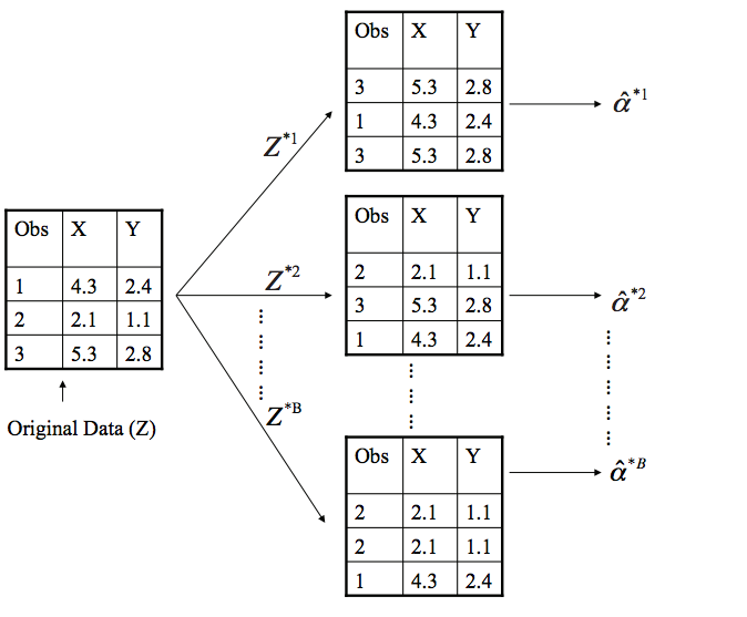
Bootstrapping involves repeatedly drawing independent samples from our data set (Z) to create bootstrap data sets (). This sample is performed with replacement, which means that the same observation can be sampled more than once and each bootstrap sample () will have the same number of observations as the original data set.
The basic idea of bootstrapping is that inference about a population from sample data, can be modelled by resampling the sample data and performing inference about a sample from resampled data (resampled → sample → population).
The bootstrap process begins with a statistic that we are interested in (). Some large number (B) of bootstrap samples are independently drawn. Each bootstrap sample is used to compute this statistic (). We can then use all the bootstrapped data sets to compute the standard error of this desired statistic
Thus, serves as an estimate of the standard error of estimated from the original data set.
The first objective in bootstrapping is to create your B bootstrap samples. We can use rsample::bootstrap to create an object that contains B resamples of the original data.
# reproducibility
set.seed(124)

# create 10 bootstap samples
(bt_samples <- bootstraps(attrition, times = 10))
## # Bootstrap sampling
## # A tibble: 10 x 2
##    splits       id
##    <list>       <chr>
##  1 <S3: rsplit> Bootstrap01
##  2 <S3: rsplit> Bootstrap02
##  3 <S3: rsplit> Bootstrap03
##  4 <S3: rsplit> Bootstrap04
##  5 <S3: rsplit> Bootstrap05
##  6 <S3: rsplit> Bootstrap06
##  7 <S3: rsplit> Bootstrap07
##  8 <S3: rsplit> Bootstrap08
##  9 <S3: rsplit> Bootstrap09
## 10 <S3: rsplit> Bootstrap10
The bootstrap samples are stored in data-frame-like tibble object where each bootstrap is nested in the splits column. We can access each bootstrap sample just as you would access parts of a list. Here, we access the first bootstrap sample stored in bt_samples$splits[[1]]. The <1470/530/1470> indicates that 1470 observations are in the bootstrap sample, 530 observations were not sampled in this bootstrap sample (meaning observations were sample 1 or more times to make the 1470 observations in the bootstrap sample), and the last 1470 indicates the total number of observations in the original data set. Remember, when performing bootstrap sampling, each bootstrap sample will always contain the same number of observations as the original data set. To extract the first bootstrap sample we can use rsample::analysis.
# observation split
bt_samples$splits[[1]]
## <1470/530/1470>

# exctract the first bootstrap sample
analysis(bt_samples$splits[[1]]) %>% as_tibble()
## # A tibble: 1,470 x 31
##      Age Attr… Busi… Dail… Depa… Dist… Educ… Educ… Envi… Gend… Hour… JobI…
##  * <int> <fct> <fct> <int> <fct> <int> <ord> <fct> <ord> <fct> <int> <ord>
##  1    56 Yes   Trav…   441 Rese…    14 Mast… Life… Medi… Fema…    72 High
##  2    32 No    Trav…   859 Rese…     4 Bach… Life… High  Fema…    98 Medi…
##  3    34 No    Trav…   216 Sales     1 Mast… Mark… Medi… Male     75 Very…
##  4    34 No    Trav…  1111 Sales     8 Coll… Life… High  Fema…    93 High
##  5    39 Yes   Trav…  1162 Sales     3 Coll… Medi… Very… Fema…    41 High
##  6    46 No    Trav…  1009 Rese…     2 Bach… Life… Low   Male     51 High
##  7    53 No    Trav…  1223 Rese…     7 Coll… Medi… Very… Fema…    50 High
##  8    50 No    Trav…   939 Rese…    24 Bach… Life… Very… Male     95 High
##  9    41 No    Trav…   337 Sales     8 Bach… Mark… High  Fema…    54 High
## 10    60 No    Trav…   422 Rese…     7 Bach… Life… Low   Fema…    41 High
## # ... with 1,460 more rows, and 19 more variables: JobLevel <int>, JobRole
## #   <fctr>, JobSatisfaction <ord>, MaritalStatus <fctr>, MonthlyIncome
## #   <int>, MonthlyRate <int>, NumCompaniesWorked <int>, OverTime <fctr>,
## #   PercentSalaryHike <int>, PerformanceRating <ord>,
## #   RelationshipSatisfaction <ord>, StockOptionLevel <int>,
## #   TotalWorkingYears <int>, TrainingTimesLastYear <int>, WorkLifeBalance
## #   <ord>, YearsAtCompany <int>, YearsInCurrentRole <int>,
## #   YearsSinceLastPromotion <int>, YearsWithCurrManager <int>
So we have successfully created bootstrap samples and we know how to access each sample. Now its time to apply a function iteratively over each bootstrap sample to compute our desired statistic.
Assume we wanted to understand the difference in income for employees that churn versus those that do not. As discussed in the multivariate statistical inference tutorial we can use the two-sample t-test to compare the difference in mean income. But what if we want to compare the difference in median income? Or the difference in the 95th percentile income?
There is no simple test statistic to perform these comparisons; however, we can use bootstrapping to get a better understanding of these estimates and their standard errors. First, we’ll create a function that computes the difference in median monthly incomes between employees that churn versus those that do not.
statistic <- function(splits) {
  x <- analysis(splits)
  median_yes <- median(x$MonthlyIncome[x$Attrition == "Yes"])
  median_no <- median(x$MonthlyIncome[x$Attrition == "No"])
  median_yes - median_no
}
The above function takes an individual bootstrap sample (i.e. split) and computes the difference in median income. Now let’s create our bootstrap samples. There is no concrete number of bootstrap samples you should use but a good rule of thumb is to use at least 500 when computing a measure of central tendency and at least 1000 when computing an extreme value such as the 95th percentile.1 With today’s modern computing power, my default is to use a minimum of 2000.
set.seed(123)
bt_samples <- bootstraps(attrition, times = 2000)
We can now iterate over each bootstrap sample and apply our statistic. Here, we use map_dbl, which comes from the purrr package and is part of the tidyverse, to iterate over each sample and compute the difference in median incomes. The results show a slightly bimodal and skewed distribution.
# iterate over each bootstrap sample and compute statistic
bt_samples$wage_diff <- map_dbl(bt_samples$splits, statistic)

# plot distribution
ggplot(bt_samples, aes(x = wage_diff)) +
  geom_line(stat = "density", adjust = 1.25) +
  xlab("Difference in Median Monthly Income (Attrition minus Non-Attrition)")
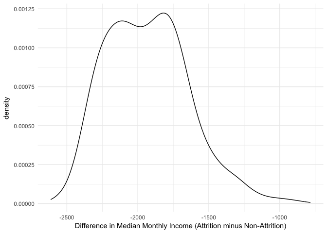
We see that across all bootstrap samples, this statistic ranges from about -2500 to -1000. We can compute the confidence interval by taking the percentiles of the bootstrap distribution. We see that the median difference is -$1,949 with a 95% confidence interval between -$2,355 and -$1,409.
quantile(bt_samples$wage_diff, probs = c(.05, .5, .95))
##        5%       50%       95%
## -2355.050 -1948.750 -1409.475
Consequently, we can be 95% confident that, on average, employees that churn are paid less than employees that do not churn (approximately -$2,355 to -$1,409 less).
Bootstrapping has many useful applications ranging from simple parameter estimates to being incorporated into modeling approaches (i.e. Random Forests). You can learn more about boostrapping, and its application in R, with the following resources: