
Machine learning algorithms typically search for the optimal representation of data using some feedback signal (aka objective/loss function). However, most machine learning algorithms only have the ability to use one or two layers of data transformation to learn the output representation. As data sets continue to grow in the dimensions of the feature space, finding the optimal output representation with a shallow model is not always possible. Deep learning provides a multi-layer approach to learn data representations, typically performed with a multi-layer neural network. Like other machine learning algorithms, deep neural networks (DNN) perform learning by mapping features to targets through a process of simple data transformations and feedback signals; however, DNNs place an emphasis on learning successive layers of meaningful representations. Although an intimidating subject, the overarching concept is rather simple and has proven highly successful in predicting a wide range of problems (i.e. image classification, speech recognition, autonomous driving). This tutorial will teach you the fundamentals of building a feedfoward deep learning model.
This tutorial serves as an introduction to feedforward DNNs and covers:
h2o and caret.This tutorial will use a few supporting packages but the main emphasis will be on the keras package. For more information on installing both CPU and GPU-based Keras and TensoFlow capabilities, visit keras.rstudio.com.
library(keras)
To illustrate various DNN concepts we will use the Ames Housing data that has been included in the AmesHousing package. However, a few important items need to be pointed out.
model.matrix.# one hot encode --> we use model.matrix(...)[, -1] to discard the intercept
data_onehot <- model.matrix(~ ., AmesHousing::make_ames())[, -1] %>% as.data.frame()
# Create training (70%) and test (30%) sets for the AmesHousing::make_ames() data.
# Use set.seed for reproducibility
set.seed(123)
split <- rsample::initial_split(data_onehot, prop = .7, strata = "Sale_Price")
train <- rsample::training(split)
test <- rsample::testing(split)
# Create & standardize feature sets
# training features
train_x <- train %>% dplyr::select(-Sale_Price)
mean <- colMeans(train_x)
std <- apply(train_x, 2, sd)
train_x <- scale(train_x, center = mean, scale = std)
# testing features
test_x <- test %>% dplyr::select(-Sale_Price)
test_x <- scale(test_x, center = mean, scale = std)
# Create & transform response sets
train_y <- log(train$Sale_Price)
test_y <- log(test$Sale_Price)
# zero variance variables (after one hot encoded) cause NaN so we need to remove
zv <- which(colSums(is.na(train_x)) > 0, useNames = FALSE)
train_x <- train_x[, -zv]
test_x <- test_x[, -zv]
# What is the dimension of our feature matrix?
dim(train_x)
## [1] 2054 299
dim(test_x)
## [1] 876 299
Neural networks originated in the computer science field to answer questions that normal statistical approaches were not designed to answer. A common example you will find is, assume we wanted to analyze hand-written digits and predict the numbers written. This was a problem presented to AT&T Bell Lab’s to help build automatic mail-sorting machines for the USPS.1
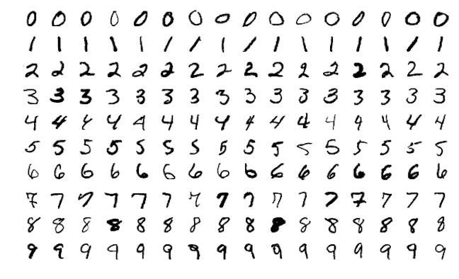
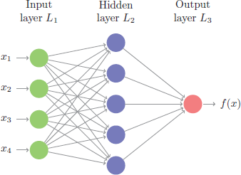
This problem is quite unique because many different features of the data can be represented. As humans, we look at these numbers and consider features such as angles, edges, thickness, completeness of circles, etc. We interpret these different representations of the features and combine them to recognize the digit. In essence, neural networks perform the same task albeit in a far simpler manner than our brains. At their most basic levels, neural networks have an input layer, hidden layer, and output layer. The input layer reads in data values from a user provided input. Within the hidden layer is where a majority of the learning takes place, and the output layer projects the results.
Although simple on the surface, historically the magic being performed inside the neural net required lots of data for the neural net to learn and was computationally intense; ultimately making neural nets impractical. However, in the last decade advancements in computer hardware (off the shelf CPUs became faster and GPUs were created) made computation more practical, the growth in data collection made them more relevant, and advancements in the underlying algorithms made the depth (number of hidden layers) of neural nets less of a constraint. These advancements have resulted in the ability to run very deep and highly parameterized neural networks, which have become known as deep neural networks (DNNs).
These DNNs allow for very complex representations of data to be modeled, which has opened the door to analyzing high-dimensional data (i.e. images, videos). In traditional machine learning approaches, features of the data need to be defined prior to modeling. One can only imagine trying to create the features for the digit recognition problem above. However, with DNNs, the hidden layers provide the means to auto-identify features. A simple way to think of this is to go back to our digit recognition problem. The first hidden layer may learn about the angles of the line, the next hidden layer may learn about the thickness of the lines, the next learns the location and completeness of the circles, etc. Aggregating these different attributes together by linking the layers allows the model to predict what digit each image is based on its features.
This is the reason that DNNs are so popular for very complex problems where feature engineering is impossible (i.e. image classification, facial recognition). However, at their core, DNNs perform successive non-linear transformations across each layer, allowing DNNs to model very complex and non-linear relationships. This can make DNNs suitable machine learning approaches for traditional regression and classification problems as well. But it is important to keep in mind that deep learning thrives when dimensions of your data are sufficiently large. As the number of observations (n) and feature inputs (p) decrease, traditional shallow machine learning approaches tend to perform just as well, if not better, and are more efficient.
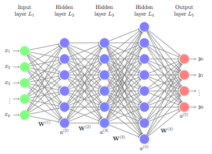
Multiple DNN models exist and, as interest and investment in this area have increased, expansions of DNN models have flurished. For example, convolutional neural networks (CNN or ConvNet) have wide applications in image and video recognition, recurrent neural networks (RNN) are used with speech recognition, and long short-term memory neural networks (LTSM) are advancing automated robotics and machine translation. However, fundamental to all these methods is the feedforward neural net (aka multilayer perceptron). Feedforward DNNs are densely connected layers where inputs influence each successive layer which then influences the final output layer.
To build a feedforward DNN we need 4 key components:
The next few sections will walk you through each of these components to build a feedforward DNN for our Ames housing data.
When developing the network architecture for a feedforward DNN, you really only need to worry about two features: (1) layers and nodes, (2) activation.
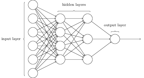
The layers and nodes are the building blocks of our model and they decide how complex your network will be. Layers are considered dense (fully connected) where all the nodes in each successive layer are connected. Consequently, the more layers and nodes you add the more opportunities for new features to be learned (commonly referred to as the model’s capacity). Beyond the input layer, which is just our predictor variables, there are two main type of layers to consider: hidden layers and an output layer.
There is no well defined approach for selecting the number of hidden layers and nodes, rather, these are the first of many tuning parameters. Typically, with regular rectangular data (think normal data frames in R), 2-5 hidden layers is sufficient. And the number of nodes you incorporate in these hidden layers is largely determined by the number of features in your data. Often, the number of nodes in each layer is equal to or less than the number of features but this is not a hard requirement. At the end of the day, the number of hidden layers and nodes in your network will drive the computational burden of your model. Consequently, the goal is to find the simplest model with optimal performance.
The output layer is driven by the type of modeling you are performing. For regression problems, your output layer will contain one node because that one node will predict a continuous numeric output. Classification problems are different. If you are predicting a binary output (True/False, Win/Loss), your output layer will still contain only one node and that node will predict the probability of success (however you define success). However, if you are predicting a multinomial output, the output layer will contain the same number of nodes as the number of classes being predicted. For example, in our digit recognition problem we would be predicting 10 classes (0-9); therefore, the output layer would have 10 nodes and the output would provide the probability of each class.
For our Ames data, to develop our network keras applies a layering approach. First, we initiate our sequential feedforward DNN architecture with keras_model_sequential and then add our dense layers. This example creates two hidden layers, the first with 10 nodes and the second with 5, followed by our output layer with one node. One thing to point out, the first layer needs the input_shape argument to equal the number of features in your data; however, the successive layers are able to dynamically interpret the number of expected inputs based on the previous layer.
model <- keras_model_sequential() %>%
  layer_dense(units = 10, input_shape = ncol(train_x)) %>%
  layer_dense(units = 5) %>%
  layer_dense(units = 1)
A key component with neural networks is what’s called activation. In the human body, the biologic neuron receives inputs from many adjacent neurons. When these inputs accumulate beyond a certain threshold the neuron is activated suggesting there is a signal. DNNs work in a similar fashion.
As stated previously, each node is connected to all the nodes in the previous layer. Each connection gets a weight and then that node adds all the incoming inputs multiplied by its corresponding connection weight (plus an extra bias () but don’t worry about that right now). The summed total of these inputs become an input to an activation function.
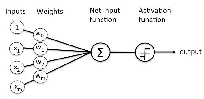
The activation function is simply a mathematical function that determines if there is enough informative input at a node to fire a signal to the next layer. There are multiple activation functions to choose from but the most common ones include:
When using rectangular data such as our Ames data, the most common approach is to use ReLU activation functions in the hidden layers. The ReLU activation function is simply taking the summed weighted inputs and transforming them to a 0 (not fire) or 1 (fire) if there is enough signal. For the output layers we use the linear activation function for regression problems and the sigmoid activation function for classification problems as this will provide the probability of the class (multinomial classification problems commonly us the softmax activation function).
To implement activation functions into our layers we simply incorporate the activation argument. For the two hidden layers we add the ReLU activation function and for the output layer we do not specify an activation function because the the default is a linear activation. Note that if we were doing a classification problem we would incorporate activation = sigmoid into the final layer_dense function call.
model <- keras_model_sequential() %>%
  layer_dense(units = 10, activation = "relu", input_shape = ncol(train_x)) %>%
  layer_dense(units = 5, activation = "relu") %>%
  layer_dense(units = 1)
We have created our basic network architecture two hidden layers with 10 and 5 nodes respectively with both hidden layers using ReLU activation functions. Next, we need to incorporate a feedback mechanism to help our model learn.
On the first model run (or forward pass), the DNN will select a batch of observations, randomly assign weights across all the node connections, and predict the output. The engine of neural networks is how it assesses its own accuracy and automatically adjusts the weights across all the node connections to try improve that accuracy. This process is called backpropagation. To perform backpropagation we need two things:
First, you need to establish an objective (loss) function to measure performance. For regression problems this is often the mean squared error (MSE) and for classification problems it is commonly binary and multi-categorical cross entropy. DNNs can have multiple loss functions but we’ll just focus on using one.
On each forward pass the DNN will measure its performance based on the loss function chosen. The DNN will then work backwards through the layers, compute the gradient2 of the loss with regards to the network weights, adjust the weights a little in the opposite direction of the gradient, grab another batch of observations to run through the model, …rinse and repeat until the loss function is minimized. This process is known as mini-batch stochastic gradient descent3 (mini-batch SGD). There are several variants of mini-batch SGD algorithms; they primarily differ in how fast they go down the gradient descent (known as learning rate). This gets more technical than we have time for in this post so I will leave it to you to learn the differences and appropriate scenarios to adjust this parameter.4 For now, realize that sticking with the default RMSProp optimizer will be sufficient for most normal regression and classification problems. However, in the tuning section I will show you how to adjust the learning rate, which can help you from getting stuck in a local optima of your loss function.
To incorporate the backpropagation piece of our DNN we add compile to our code sequence. In addition to the optimizer and loss function arguments, we can also identify one or more metrics in addition to our loss function to track and report.
model <- keras_model_sequential() %>%

  # network architecture
  layer_dense(units = 10, activation = "relu", input_shape = ncol(train_x)) %>%
  layer_dense(units = 5, activation = "relu") %>%
  layer_dense(units = 1) %>%

  # backpropagation
  compile(
    optimizer = "rmsprop",
    loss = "mse",
    metrics = c("mae")
  )
We’ve created a base model, now we just need to train it with our data. To do so we feed our model into a fit function along with our training data. We also provide a few other arguments that are worth mentioning:
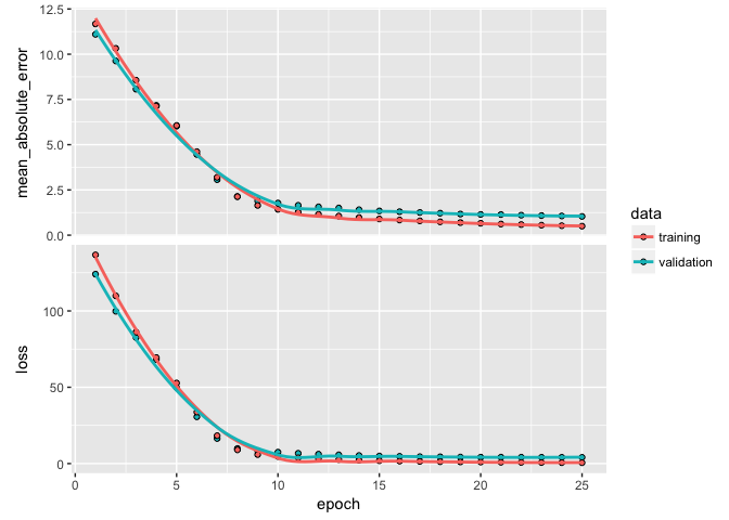
batch_size: As I mentioned in the last section, the DNN will take a batch of data to run through the mini-batch SGD process. Batch sizes can be between 1 and several hundred. Small values will be more computationally burdomesome while large values provide less feedback signal. Typically, 32 is a good size to start with and the values are typically provided as a power of two that fit nicely into the memory requirements of the GPU or CPU hardware like 32, 64, 128, 256, and so on.epochs: An epoch describes the number of times the algorithm sees the entire data set. So, each time the algorithm has seen all samples in the dataset, an epoch has completed. In our training set, we have 2054 observations so running batches of 32 will require 64 passes for one epoch. The more complex the features and relationships in your data, the more epochs you will require for your model to learn, adjust the weights, and minimize the loss function.validation_split: Allows us to perform cross-validation. The model will hold out XX% of the data so that we can compute a more accurate estimate of an out-of-sample error rate.verbose: I set this to FALSE for creating this tutorial; however, when TRUE you will see a live update of the loss function in your RStudio IDE.Plotting our output shows how our loss function (and specified metrics) improve for each epoch. We see that our MSE flatlines around the 10th epoch.
model <- keras_model_sequential() %>%

  # network architecture
  layer_dense(units = 10, activation = "relu", input_shape = ncol(train_x)) %>%
  layer_dense(units = 5, activation = "relu") %>%
  layer_dense(units = 1) %>%

  # backpropagation
  compile(
    optimizer = "rmsprop",
    loss = "mse",
    metrics = c("mae")
  )

# train our model
learn <- model %>% fit(
  x = train_x,
  y = train_y,
  epochs = 25,
  batch_size = 32,
  validation_split = .2,
  verbose = FALSE
)

learn
## Trained on 1,643 samples, validated on 411 samples (batch_size=32, epochs=25)
## Final epoch (plot to see history):
## val_mean_absolute_error: 1.034
##                val_loss: 4.078
##     mean_absolute_error: 0.4967
##                    loss: 0.5555
plot(learn)
Now that we have an understanding of producing and running our DNN model, the next task is to find an optimal model by tuning different parameters. There are many ways to tune a DNN. Typically, the tuning process follows these general steps; however, there is often a lot of iteration among these:
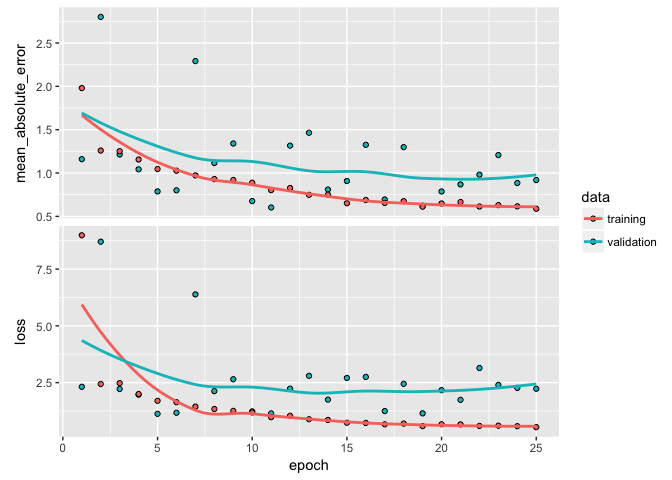
Typically, we start with a high capacity model (several layers and nodes) to deliberately overfit the data. When do we know we’ve overfit? When we start to see our validation metrics deteriate we can be confident we’ve overfit. For example, here is a highly parameterized model with 3 layers and 500, 250, and 125 nodes per layer respectively. Our output shows high variability in our validation metrics.
model <- keras_model_sequential() %>%

  # network architecture
  layer_dense(units = 500, activation = "relu", input_shape = ncol(train_x)) %>%
  layer_dense(units = 250, activation = "relu", input_shape = ncol(train_x)) %>%
  layer_dense(units = 125, activation = "relu") %>%
  layer_dense(units = 1) %>%

  # backpropagation
  compile(
    optimizer = "rmsprop",
    loss = "mse",
    metrics = c("mae")
  )

# train our model
learn <- model %>% fit(
  x = train_x,
  y = train_y,
  epochs = 25,
  batch_size = 32,
  validation_split = .2,
  verbose = FALSE
)

plot(learn)
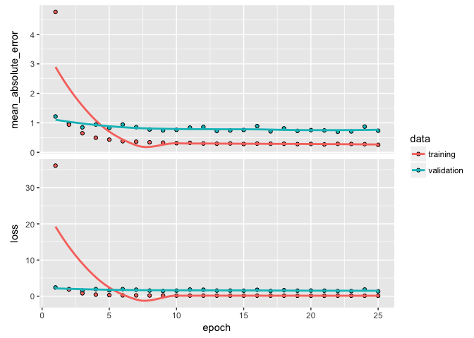
Once we’ve overfit, we can reduce our layers and nodes until we see improvement in our validation metrics. Not only do we want to see stable validation metrics, we also want to find the model capacity that minimizes overfitting. Here, I find that 2 layers with 100 and 50 nodes respectively does a pretty good job of stabilizing our errors and minimizing our metrics and overfitting.
model <- keras_model_sequential() %>%

  # network architecture
  layer_dense(units = 100, activation = "relu", input_shape = ncol(train_x)) %>%
  layer_dense(units = 50, activation = "relu") %>%
  layer_dense(units = 1) %>%

  # backpropagation
  compile(
    optimizer = "rmsprop",
    loss = "mse",
    metrics = c("mae")
  )

# train our model
learn <- model %>% fit(
  x = train_x,
  y = train_y,
  epochs = 25,
  batch_size = 32,
  validation_split = .2,
  verbose = FALSE
)

plot(learn)
If you notice your loss function is still decreasing in the last epoch then you will want to increase the number of epochs. Alternatively, if your epochs flatline early then there is no reason to run so many epochs as you are just using extra computational energy with no gain. We can add a callback function inside of fit to help with this. There are multiple callbacks to help automate certain tasks. One such callback is early stopping, which will stop training if the loss function does not improve for a specified number of epochs.
Here, I incorporate callback_early_stopping(patience = 2) to stop training if the MSE has not improved for 3 epochs.
model <- keras_model_sequential() %>%
# network architecture
layer_dense(units = 100, activation = "relu", input_shape = ncol(train_x)) %>%
layer_dense(units = 50, activation = "relu") %>%
layer_dense(units = 1) %>%
# backpropagation
compile(
optimizer = "rmsprop",
loss = "mse",
metrics = c("mae")
)
# train our model
learn <- model %>% fit(
x = train_x,
y = train_y,
epochs = 25,
batch_size = 32,
validation_split = .2,
verbose = FALSE,
callbacks = list(
callback_early_stopping(patience = 2)
)
)
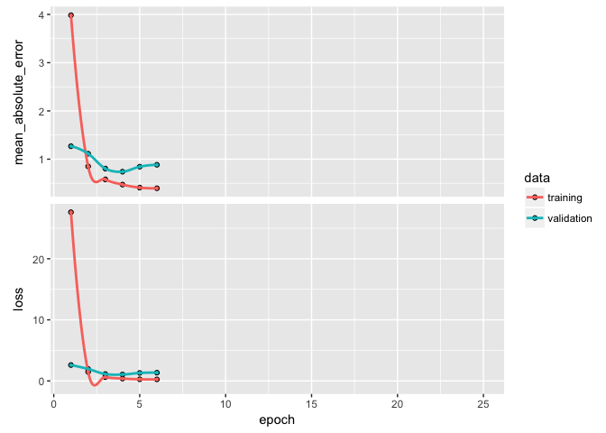
learn
## Trained on 1,643 samples, validated on 411 samples (batch_size=32, epochs=6)
## Final epoch (plot to see history):
## val_mean_absolute_error: 0.8835
## val_loss: 1.353
## mean_absolute_error: 0.397
## loss: 0.2517
plot(learn)
So far we have normalized our data before feeding it into our model. But data normalization should be a concern after every transformation operated by the network. Batch normalization is a recent advancement that adaptively normalizes data even as the mean and variance change over time during training. The main effect of batch normalization is that it helps with gradient propogation, which allows for deeper networks. Consequently, as the depth of your DNN increases, batch normalization becomes more important.
We add batch normalization with layer_batch_normalization and we see an improvement in our performance metrics and our overfitting has been further minimized.
model <- keras_model_sequential() %>%
# network architecture
layer_dense(units = 100, activation = "relu", input_shape = ncol(train_x)) %>%
layer_batch_normalization() %>%
layer_dense(units = 50, activation = "relu") %>%
layer_batch_normalization() %>%
layer_dense(units = 1) %>%
# backpropagation
compile(
optimizer = "rmsprop",
loss = "mse",
metrics = c("mae")
)
# train our model
learn <- model %>% fit(
x = train_x,
y = train_y,
epochs = 25,
batch_size = 32,
validation_split = .2,
verbose = FALSE,
callbacks = list(
callback_early_stopping(patience = 2)
)
)
learn
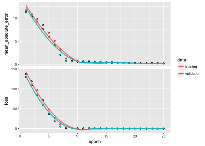
## Trained on 1,643 samples, validated on 411 samples (batch_size=32, epochs=25)
## Final epoch (plot to see history):
## val_mean_absolute_error: 0.2016
## val_loss: 0.07756
## mean_absolute_error: 0.1786
## loss: 0.05482
plot(learn)
Dropout is one of the most effective and commonly used approaches to prevent overfitting in neural networks. Dropout randomly drops out (setting to zero) a number of output features in a layer during training. By randomly removing different nodes, we help prevent the model from fitting patterns to happenstance patterns (noise) that are not significant. We apply drop out with layer_dropout.
A typical dropout rate is 0.2 and 0.5. In this example I drop out 20% of the inputs going into each layer. In this example we do not see improvement in our model’s performance or in overfitting so we’ll drop dropout5 from future models.
model <- keras_model_sequential() %>%
# network architecture
layer_dense(units = 100, activation = "relu", input_shape = ncol(train_x)) %>%
layer_batch_normalization() %>%
layer_dropout(rate = 0.2) %>%
layer_dense(units = 50, activation = "relu") %>%
layer_batch_normalization() %>%
layer_dropout(rate = 0.2) %>%
layer_dense(units = 1) %>%
# backpropagation
compile(
optimizer = "rmsprop",
loss = "mse",
metrics = c("mae")
)
# train our model
learn <- model %>% fit(
x = train_x,
y = train_y,
epochs = 25,
batch_size = 32,
validation_split = .2,
verbose = FALSE,
callbacks = list(
callback_early_stopping(patience = 2)
)
)
learn
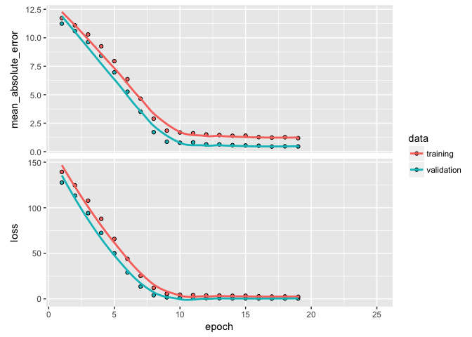
## Trained on 1,643 samples, validated on 411 samples (batch_size=32, epochs=19)
## Final epoch (plot to see history):
## val_mean_absolute_error: 0.4557
## val_loss: 0.4161
## mean_absolute_error: 1.185
## loss: 2.247
plot(learn)
In a previous tutorial, we discussed the idea of regularization. The same idea can be applied in DNNs where we put constraints on the size that the weights can take. In DNNs, the most common regularization is the norm, which is called weight decay in the context of neural networks. Regularization of weights will force small signals (noise) to have weights nearly equal to zero and only allow signals with consistently strong signals to have relatively larger weights.
We apply regularization with a kernel_regularizer argument in our layer_dense functions. In this example I add the norm regularizer with a multiplier of 0.001, which means every weight coefficient in the layer will be multiplied by 0.001. We could also add an regularization or a combination of and (aka elastic net) with regularizer_l1 and regularizer_l1_l2 respectively. Here, weight decay doesn’t really improve our performance metrics but it does help a little in reducing overfitting.
model <- keras_model_sequential() %>%
# network architecture
layer_dense(units = 100, activation = "relu", input_shape = ncol(train_x),
kernel_regularizer = regularizer_l2(0.001)) %>%
layer_batch_normalization() %>%
layer_dense(units = 50, activation = "relu",
kernel_regularizer = regularizer_l2(0.001)) %>%
layer_batch_normalization() %>%
layer_dense(units = 1) %>%
# backpropagation
compile(
optimizer = "rmsprop",
loss = "mse",
metrics = c("mae")
)
# train our model
learn <- model %>% fit(
x = train_x,
y = train_y,
epochs = 25,
batch_size = 32,
validation_split = .2,
verbose = FALSE,
callbacks = list(
callback_early_stopping(patience = 2)
)
)
learn
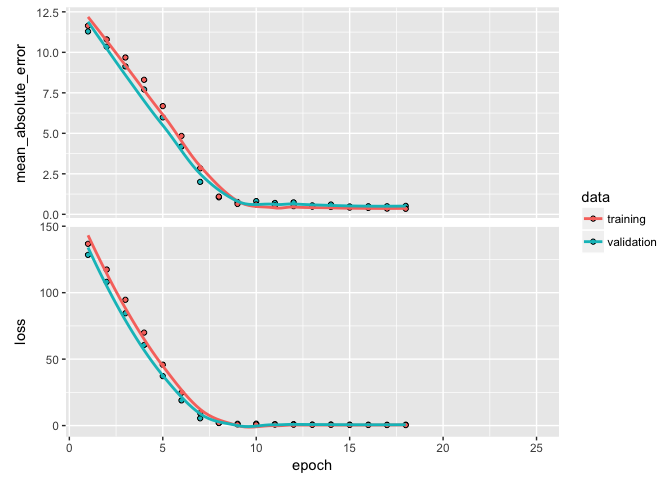
## Trained on 1,643 samples, validated on 411 samples (batch_size=32, epochs=18)
## Final epoch (plot to see history):
## val_mean_absolute_error: 0.5196
## val_loss: 0.6465
## mean_absolute_error: 0.342
## loss: 0.3858
plot(learn)
Another issue to be concerned with is whether or not we are finding a global minimum versus a local minimum with our loss value. The mini-batch SGD optimizer we use will take incremental steps down our loss gradient until it no longer experiences improvement. The size of the incremental steps (aka learning rate) will determine if we get stuck in a local minimum instead of making our way to the global minimum.
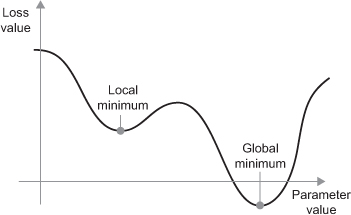
There are two ways to circumvent this problem:
Here, we’ll just focus on #2. We can incorporate another callback function to automatically adjust the learning rate upon plateauing. By default, callback_reduce_lr_on_plateau will divide the learning rate by 10 if the validation loss value does not improve for 10 epochs.
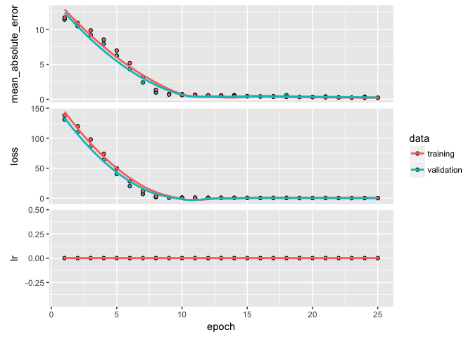
We do not see substantial improvement in our validation loss, which suggests we are likely not running into problems with a local minimum.
model <- keras_model_sequential() %>%

  # network architecture
  layer_dense(units = 100, activation = "relu", input_shape = ncol(train_x),
              kernel_regularizer = regularizer_l2(0.001)) %>%
  layer_batch_normalization() %>%
  layer_dense(units = 50, activation = "relu",
              kernel_regularizer = regularizer_l2(0.001)) %>%
  layer_batch_normalization() %>%
  layer_dense(units = 1) %>%

  # backpropagation
  compile(
    optimizer = "rmsprop",
    loss = "mse",
    metrics = c("mae")
  )

# train our model
learn <- model %>% fit(
  x = train_x,
  y = train_y,
  epochs = 25,
  batch_size = 32,
  validation_split = .2,
  verbose = FALSE,
  callbacks = list(
    callback_early_stopping(patience = 2),
    callback_reduce_lr_on_plateau()
  )
)

learn
## Trained on 1,643 samples, validated on 411 samples (batch_size=32, epochs=25)
## Final epoch (plot to see history):
## val_mean_absolute_error: 0.2325
##                val_loss: 0.2685
##                      lr: 0.001
##     mean_absolute_error: 0.2119
##                    loss: 0.2482

plot(learn)
So, we have found a pretty good model. Next we want to predict on our test data to produce our generalized expectation of error. We can use predict to predict our log sales prices for the test set.
model %>% predict(test_x[1:10,])
##           [,1]
##  [1,] 11.65819
##  [2,] 12.42168
##  [3,] 12.21052
##  [4,] 12.70359
##  [5,] 13.58570
##  [6,] 13.52976
##  [7,] 12.80696
##  [8,] 12.00162
##  [9,] 11.45837
## [10,] 11.67073
We can also use evaluate to get the same performance metrics we were assessing while training the data. We see that our test MSE is 0.278 and MAE is 0.30, both of which align closely with our last model so we are not overfitting.
(results <- model %>% evaluate(test_x, test_y))
## $loss
## [1] 0.2781004
##
## $mean_absolute_error
## [1] 0.3045773
However, if we transform our results back to the original unit level we see that our RMSE suggests that, on average, our estimates are about $67K off from the actual sales price. Considering the mean sales price is about $180K, this is still a sizeable error. In fact, when we use a simple lasso linear model we achieve an RMSE of $24K. So this is a good example of where a highly parameterized non-linear DNN does not perform better than a simpler, parameter-constrained linear model.
model %>%
  predict(test_x) %>%
  broom::tidy() %>%
  dplyr::mutate(
    truth = test_y,
    pred_tran = exp(x),
    truth_tran = exp(truth)
    ) %>%
   yardstick::rmse(truth_tran, pred_tran)
## [1] 67230.07
keras is not the only package that can perform deep learning. The following also shows how to implement with the popular caret and h2o packages. For brevity, I show the code but not the output.
caretcaret has several options for developing a feedforward neural network. You can leverage R packages such as mxnet, nnet, mlpML, etc. You can see all the options here. The primary downfall of using caret is the inconsistencies in the tuning parameters across the different packages. Some you can adjust the number of hidden layers and nodes within the layers, others only allow 1 or 2 hidden layers. Some allow you to adjust the learning rate and incorporate dropout while others do not.
The mxnet package is one of the more flexible neural network packages. Here I create a similar model structure to what I created above; however, I am not able to adjust the mini-batch SGD optimizer nor incorporate batch normalization which helped reduce our MSE and overfitting in earlier examples.
library(caret)

# specify tuning parameters
mlp_grid <- expand.grid(
  layer1 = 100,
  layer2 = 50,
  layer3 = 1,
  learning.rate = 0.05,
  momentum = 0.01,
  dropout = 0,
  activation = "relu"
  )

# train DNN model
mlp_fit <- caret::train(
  x = train_x,
  y = train_y,
  method = "mxnet",
  preProc =  NULL,
  trControl = trainControl(method = "cv"),
  tuneGrid = mlp_grid
  )

mlp_fit
h2oh2o.deeplearning performs multi-layer feedforward DNNs trained with stochastic gradient descent using back-propagation. It provides similar advanced features as the keras package, such as adaptive learning rate, rate annealing, momentum training, dropout, L1 or L2 regularization, checkpointing, etc.
# h2o package
library(h2o)
h2o.init()

# convert data to h2o object --> here we use our original data as h2o will
# perform one-hot encoding and standardization for us.
ames_h2o <- train %>%
  mutate(Sale_Price_log = log(Sale_Price)) %>%
  as.h2o()

# set the response column to Sale_Price_log
response <- "Sale_Price_log"

# set the predictor names
predictors <- setdiff(colnames(train), "Sale_Price")

# train a model with defined parameters
model <- h2o.deeplearning(
  x = predictors,
  y = response,
  training_frame = ames_h2o,
  nfolds = 10,                                 # 10-fold CV
  keep_cross_validation_predictions = TRUE,    # retain CV prediction values
  distribution = "gaussian",                   # output is continuous
  activation = "Rectifier",                    # use ReLU in hidden layers
  hidden = c(100, 50),                         # two hidden layers
  epochs = 25,                                 # number of epochs to perform
  stopping_metric = "MSE",                     # loss function is MSE
  stopping_rounds = 5,                         # allows early stopping
  l2 = 0.001,                                  # L2 norm weight regularization
  mini_batch_size = 32                         # batch sizes
  )

# check out results
model
plot(model, timestep = "epochs", metric = "rmse")
print(h2o.mse(model, xval = TRUE))
print(h2o.rmse(model, xval = TRUE))

# variable importance
h2o.varimp_plot(model, 20)
h2o.partialPlot(model, ames_h2o, cols = "Gr_Liv_Area")
Furthermore, it also provides grid search capabilities that help to automate the tuning process. This is a feature not provided by keras at this time.
# create hyperparameter grid search
hyper_params <- list(
  activation = c("Rectifier", "RectifierWithDropout", "Maxout", "MaxoutWithDropout"),
  l1 = c(0, 0.00001, 0.0001, 0.001, 0.01, 0.1),
  l2 = c(0, 0.00001, 0.0001, 0.001, 0.01, 0.1)
  )

# For a larger search space we can use random grid search
search_criteria <- list(strategy = "RandomDiscrete", max_runtime_secs = 120)

# Rather than comparing models by using cross-validation (which is “better” but
# takes longer), we will simply partition our training set into two pieces – one
# for training and one for validiation.
splits <- h2o.splitFrame(ames_h2o, ratios = 0.8, seed = 1)

# train the grid
dl_grid <- h2o.grid(
  algorithm = "deeplearning",
  x = predictors,
  y = response,
  grid_id = "dl_grid",
  training_frame = splits[[1]],
  validation_frame = splits[[2]],
  seed = 1,
  hidden = c(100, 50),
  hyper_params = hyper_params,
  search_criteria = search_criteria
  )

# collect the results and sort by our model performance metric of choice
dl_gridperf <- h2o.getGrid(
  grid_id = "dl_grid",
  sort_by = "mse",
  decreasing = TRUE
  )
print(dl_gridperf)

# Grab the model_id for the top model, chosen by validation error
best_dl_model_id <- dl_gridperf@model_ids[[1]]
best_dl <- h2o.getModel(best_dl_model_id)

# Now let’s evaluate the model performance on a test set
ames_test <- test %>%
  mutate(Sale_Price_log = log(Sale_Price)) %>%
  as.h2o()
best_dl_perf <- h2o.performance(model = best_dl, newdata = ames_test)
h2o.mse(best_dl_perf)
This serves as an introduction to DNNs; however, it barely scratches the surface of what these models can do. Extensions of this exemplar feedforward DNN have proven to be first class predictors for image classification, video analysis, speech recognition, and other feature rich data sets. The following are great resources to learn more (listed in order of complexity):
LeCun, Y., et al. (1990). Handwritten digit recognition with a back-propagation network. In Advances in neural information processing systems (pp. 396-404).. ↩
A gradient is the generalization of the concept of derivatives applied to functions of multidimensional inputs. ↩
Its considered stochastic because a random subset (batch) of observations are drawn for each forward pass. ↩
I would start with this great overview paper of gradient descent optimization algorithms. ↩
Pun totally intended. ↩