
![]() As discussed, linear regression is a simple and fundamental approach for supervised learning. Moreover, when the assumptions required by ordinary least squares (OLS) regression are met, the coefficients produced by OLS are unbiased and, of all unbiased linear techniques, have the lowest variance. However, in today’s world, data sets being analyzed typically have a large amount of features. As the number of features grow, our OLS assumptions typically break down and our models often overfit (aka have high variance) to the training sample, causing our out of sample error to increase. Regularization methods provide a means to control our regression coefficients, which can reduce the variance and decrease out of sample error.
As discussed, linear regression is a simple and fundamental approach for supervised learning. Moreover, when the assumptions required by ordinary least squares (OLS) regression are met, the coefficients produced by OLS are unbiased and, of all unbiased linear techniques, have the lowest variance. However, in today’s world, data sets being analyzed typically have a large amount of features. As the number of features grow, our OLS assumptions typically break down and our models often overfit (aka have high variance) to the training sample, causing our out of sample error to increase. Regularization methods provide a means to control our regression coefficients, which can reduce the variance and decrease out of sample error.
This tutorial serves as an introduction to regularization and covers:
This tutorial leverages the following packages. Most of these packages are playing a supporting role while the main emphasis will be on the glmnet package.
library(rsample)  # data splitting
library(glmnet)   # implementing regularized regression approaches
library(dplyr)    # basic data manipulation procedures
library(ggplot2)  # plotting
To illustrate various regularization concepts we will use the Ames Housing data that has been included in the AmesHousing package.
# Create training (70%) and test (30%) sets for the AmesHousing::make_ames() data.
# Use set.seed for reproducibility

set.seed(123)
ames_split <- initial_split(AmesHousing::make_ames(), prop = .7, strata = "Sale_Price")
ames_train <- training(ames_split)
ames_test  <- testing(ames_split)
The objective of ordinary least squares regression is to find the plane that minimizes the sum of squared errors (SSE) between the observed and predicted response. In Figure 1, this means identifying the plane that minimizes the grey lines, which measure the distance between the observed (red dots) and predicted response (blue plane).
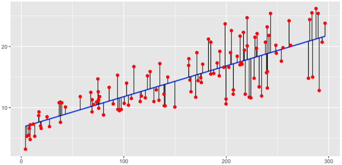
Fig.1: Fitted regression line using Ordinary Least Squares.
More formally, this objective function is written as:
The OLS objective function performs quite well when our data align to the key assumptions of OLS regression:
However, for many real-life data sets we have very wide data, meaning we have a large number of features (p) that we believe are informative in predicting some outcome. As p increases, we can quickly violate some of the OLS assumptions and we require alternative approaches to provide predictive analytic solutions. Specifically, as p increases there are three main issues we most commonly run into:
As p increases we are more likely to capture multiple features that have some multicollinearity. When multicollinearity exists, we often see high variability in our coefficient terms. For example, in our Ames data, Gr_Liv_Area and TotRms_AbvGrd are two variables that have a correlation of 0.801 and both variables are strongly correlated to our response variable (Sale_Price). When we fit a model with both these variables we get a positive coefficient for Gr_Liv_Area but a negative coefficient for TotRms_AbvGrd, suggesting one has a positive impact to Sale_Price and the other a negative impact.
# fit with two strongly correlated variables
lm(Sale_Price ~ Gr_Liv_Area + TotRms_AbvGrd, data = ames_train)
##
## Call:
## lm(formula = Sale_Price ~ Gr_Liv_Area + TotRms_AbvGrd, data = ames_train)
##
## Coefficients:
##   (Intercept)    Gr_Liv_Area  TotRms_AbvGrd
##       49953.6          137.3       -11788.2
However, if we refit the model with each variable independently, they both show a positive impact. However, the Gr_Liv_Area effect is now smaller and the TotRms_AbvGrd is positive with a much larger magnitude.
# fit with just Gr_Liv_Area
lm(Sale_Price ~ Gr_Liv_Area, data = ames_train)
##
## Call:
## lm(formula = Sale_Price ~ Gr_Liv_Area, data = ames_train)
##
## Coefficients:
## (Intercept)  Gr_Liv_Area
##       17797          108

# fit with just TotRms_Area
lm(Sale_Price ~ TotRms_AbvGrd, data = ames_train)
##
## Call:
## lm(formula = Sale_Price ~ TotRms_AbvGrd, data = ames_train)
##
## Coefficients:
##   (Intercept)  TotRms_AbvGrd
##         26820          23731
This is a common result when collinearity exists. Coefficients for correlated features become over-inflated and can fluctuate significantly. One consequence of these large fluctuations in the coefficient terms is overfitting, which means we have high variance in the bias-variance tradeoff space. Although an analyst can use tools such as variance inflaction factors (Myers, 1994) to identify and remove those strongly correlated variables, it is not always clear which variable(s) to remove. Nor do we always wish to remove variables as this may be removing signal in our data.
When the number of features exceed the number of observations (), the OLS solution matrix is not invertible. This causes significant issues because it means: (1) The least-squares estimates are not unique. In fact, there are an infinite set of solutions available and most of these solutions overfit the data. (2) In many instances the result will be computationally infeasible.
Consequently, to resolve this issue an analyst can remove variables until and then fit an OLS regression model. Although an analyst can use pre-processing tools to guide this manual approach (Kuhn & Johnson, 2013, pp. 43-47), it can be cumbersome and prone to errors.
With a large number of features, we often would like to identify a smaller subset of these features that exhibit the strongest effects. In essence, we sometimes prefer techniques that provide feature selection. One approach to this is called hard threshholding feature selection, which can be performed with linear model selection approaches. However, model selection approaches can be computationally inefficient, do not scale well, and they simply assume a feature as in or out. We may wish to use a soft threshholding approach that slowly pushes a feature’s effect towards zero. As will be demonstrated, this can provide additional understanding regarding predictive signals.
When we experience these concerns, one alternative to OLS regression is to use regularized regression (also commonly referred to as penalized models or shrinkage methods) to control the parameter estimates. Regularized regression puts contraints on the magnitude of the coefficients and will progressively shrink them towards zero. This constraint helps to reduce the magnitude and fluctuations of the coefficients and will reduce the variance of our model.
The objective function of regularized regression methods is very similar to OLS regression; however, we add a penalty parameter (P).
There are two main penalty parameters, which we’ll see shortly, but they both have a similar effect. They constrain the size of the coefficients such that the only way the coefficients can increase is if we experience a comparable decrease in the sum of squared errors (SSE). Next, we’ll explore the most common approaches to incorporate regularization.
Ridge regression (Hoerl, 1970) controls the coefficients by adding to the objective function. This penalty parameter is also referred to as “” as it signifies a second-order penalty being used on the coefficients.1
This penalty parameter can take on a wide range of values, which is controlled by the tuning parameter . When there is no effect and our objective function equals the normal OLS regression objective function of simply minimizing SSE. However, as , the penalty becomes large and forces our coefficients to zero. This is illustrated in Figure 2 where exemplar coefficients have been regularized with ranging from 0 to over 8,000 ().
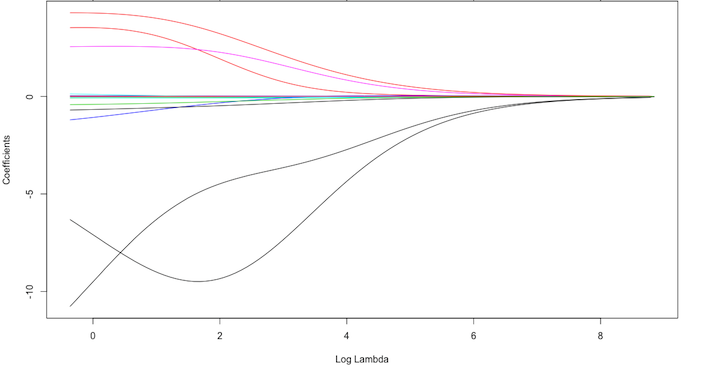
Fig.2: Ridge regression coefficients as λ grows from 0 → ∞.
Although these coefficients were scaled and centered prior to the analysis, you will notice that some are extremely large when . Furthermore, you’ll notice the large negative parameter that fluctuates until where it then continuously skrinks to zero. This is indicitive of multicollinearity and likely illustrates that constraining our coefficients with may reduce the variance, and therefore the error, in our model. However, the question remains - how do we find the amount of shrinkage (or ) that minimizes our error? We’ll answer this shortly.
To implement Ridge regression we will focus on the glmnet package (implementation in other packages are illustrated below). glmnet does not use the formula method (y ~ x) so prior to modeling we need to create our feature and target set. Furthermore, we use the model.matrix function on our feature set, which will automatically dummy encode qualitative variables (see Matrix::sparse.model.matrix for increased efficiency on large dimension data). We also log transform our response variable due to its skeweness.
# Create training and testing feature model matrices and response vectors.
# we use model.matrix(...)[, -1] to discard the intercept
ames_train_x <- model.matrix(Sale_Price ~ ., ames_train)[, -1]
ames_train_y <- log(ames_train$Sale_Price)

ames_test_x <- model.matrix(Sale_Price ~ ., ames_test)[, -1]
ames_test_y <- log(ames_test$Sale_Price)

# What is the dimension of of your feature matrix?
dim(ames_train_x)
## [1] 2054  307
To apply a ridge model we can use the glmnet::glmnet function. The alpha parameter tells glmnet to perform a ridge (alpha = 0), lasso (alpha = 1), or elastic net () model. Behind the scenes, glmnet is doing two things that you should be aware of:
glmnet performs this for you. If you standardize your predictors prior to glmnet you can turn this argument off with standardize = FALSE.glmnet will perform ridge models across a wide range of parameters, which are illustrated in the figure below.# Apply Ridge regression to ames data
ames_ridge <- glmnet(
x = ames_train_x,
y = ames_train_y,
alpha = 0
)
plot(ames_ridge, xvar = "lambda")

In fact, we can see the exact values applied with ames_ridge$lambda. Although you can specify your own values, by default glmnet applies 100 values that are data derived. Majority of the time you will have little need to adjust the default values.
We can also directly access the coefficients for a model using coef. glmnet stores all the coefficients for each model in order of largest to smallest . Due to the number of features, here I just peak at the coefficients for the Gr_Liv_Area and TotRms_AbvGrd features for the largest (279.1035) and smallest (0.02791035). You can see how the largest value has pushed these coefficients to nearly 0.
# lambdas applied to penalty parameter
ames_ridge$lambda %>% head()
## [1] 279.1035 254.3087 231.7166 211.1316 192.3752 175.2851

# coefficients for the largest and smallest lambda parameters
coef(ames_ridge)[c("Gr_Liv_Area", "TotRms_AbvGrd"), 100]
##   Gr_Liv_Area TotRms_AbvGrd
##  0.0001004011  0.0096383231
coef(ames_ridge)[c("Gr_Liv_Area", "TotRms_AbvGrd"), 1]
##   Gr_Liv_Area TotRms_AbvGrd
##  5.551202e-40  1.236184e-37
However, at this point, we do not understand how much improvement we are experiencing in our model.
Recall that is a tuning parameter that helps to control our model from over-fitting to the training data. However, to identify the optimal value we need to perform cross-validation (CV). cv.glmnet provides a built-in option to perform k-fold CV, and by default, performs 10-fold CV.
# Apply CV Ridge regression to ames data
ames_ridge <- cv.glmnet(
  x = ames_train_x,
  y = ames_train_y,
  alpha = 0
)

# plot results
plot(ames_ridge)

Our plot output above illustrates the 10-fold CV mean squared error (MSE) across the values. It illustrates that we do not see substantial improvement; however, as we constrain our coefficients with penalty, the MSE rises considerably. The numbers at the top of the plot (299) just refer to the number of variables in the model. Ridge regression does not force any variables to exactly zero so all features will remain in the model (we’ll see this change with lasso and elastic nets).
The first and second vertical dashed lines represent the value with the minimum MSE and the largest value within one standard error of the minimum MSE.
min(ames_ridge$cvm)       # minimum MSE
## [1] 0.02147691
ames_ridge$lambda.min     # lambda for this min MSE
## [1] 0.1236602

ames_ridge$cvm[ames_ridge$lambda == ames_ridge$lambda.1se]  # 1 st.error of min MSE
## [1] 0.02488411
ames_ridge$lambda.1se  # lambda for this MSE
## [1] 0.6599372
The advantage of identifying the with an MSE within one standard error becomes more obvious with the lasso and elastic net models. However, for now we can assess this visually. Here we plot the coefficients across the values and the dashed red line represents the largest that falls within one standard error of the minimum MSE. This shows you how much we can constrain the coefficients while still maximizing predictive accuracy.
ames_ridge_min <- glmnet(
  x = ames_train_x,
  y = ames_train_y,
  alpha = 0
)

plot(ames_ridge_min, xvar = "lambda")
abline(v = log(ames_ridge$lambda.1se), col = "red", lty = "dashed")

In essence, the ridge regression model has pushed many of the correlated features towards each other rather than allowing for one to be wildly positive and the other wildly negative. Furthermore, many of the non-important features have been pushed closer to zero. This means we have reduced the noise in our data, which provides us more clarity in identifying the true signals in our model.
coef(ames_ridge, s = "lambda.1se") %>%
  tidy() %>%
  filter(row != "(Intercept)") %>%
  top_n(25, wt = abs(value)) %>%
  ggplot(aes(value, reorder(row, value))) +
  geom_point() +
  ggtitle("Top 25 influential variables") +
  xlab("Coefficient") +
  ylab(NULL)

However, a ridge model will retain
The least absolute shrinkage and selection operator (lasso) model (Tibshirani, 1996) is an alternative to ridge regression that has a small modification to the penalty in the objective function. Rather than the penalty we use the following penalty in the objective function.
Whereas the ridge regression approach pushes variables to approximately but not equal to zero, the lasso penalty will actually push coefficients to zero as illustrated with Fig. 3. Thus the lasso model not only improves the model with regularization but it also conducts automated feature selection.

Fig.3: Lasso regression coefficients as λ grows from 0 → ∞.
In Fig. 3 we see that when all 15 variables are in the model, when 12 variables are retained, and when only 3 variables are retained. Consequently, when a data set has many features lasso can be used to identify and extract those features with the largest (and most consistent) signal.
Implementing lasso follows the same logic as implementing the ridge model, we just need to switch alpha = 1 within glmnet.
## Apply lasso regression to ames data
ames_lasso <- glmnet(
  x = ames_train_x,
  y = ames_train_y,
  alpha = 1
)

plot(ames_lasso, xvar = "lambda")

Our output illustrates a quick drop in the number of features retained in the lasso model as . In fact, we see several features that had very large coefficients for the OLS model (when ). As before, these features are likely highly correlated with other features in the data, causing their coefficients to be excessively large. As we constrain our model, these noisy features are pushed to zero.
However, similar to the Ridge regression section, we need to perfom CV to determine what the right value is for .
To perform CV we use the same approach as we did in the ridge regression tuning section, but change our alpha = 1. We see that we can minimize our MSE by applying approximately . Not only does this minimize our MSE but it also reduces the number of features to .
# Apply CV Ridge regression to ames data
ames_lasso <- cv.glmnet(
  x = ames_train_x,
  y = ames_train_y,
  alpha = 1
)
# plot results
plot(ames_lasso)

As before, we can extract our minimum and one standard error MSE and values.
min(ames_lasso$cvm)       # minimum MSE
## [1] 0.02275227
ames_lasso$lambda.min     # lambda for this min MSE
## [1] 0.003521887

ames_lasso$cvm[ames_lasso$lambda == ames_lasso$lambda.1se]  # 1 st.error of min MSE
## [1] 0.02562055
ames_lasso$lambda.1se  # lambda for this MSE
## [1] 0.01180396
Now the advantage of identifying the with an MSE within one standard error becomes more obvious. If we use the that drives the minimum MSE we can reduce our feature set from 307 down to less than 160. However, there will be some variability with this MSE and we can reasonably assume that we can achieve a similar MSE with a slightly more constrained model that uses only 63 features. If describing and interpreting the predictors is an important outcome of your analysis, this may significantly aid your endeavor.
ames_lasso_min <- glmnet(
  x = ames_train_x,
  y = ames_train_y,
  alpha = 1
)

plot(ames_lasso_min, xvar = "lambda")
abline(v = log(ames_lasso$lambda.min), col = "red", lty = "dashed")
abline(v = log(ames_lasso$lambda.1se), col = "red", lty = "dashed")

Similar to ridge, the lasso pushes many of the collinear features towards each other rather than allowing for one to be wildly positive and the other wildly negative. However, unlike ridge, the lasso will actually push coefficients to zero and perform feature selection. This simplifies and automates the process of identifying those feature most influential to predictive accuracy.
coef(ames_lasso, s = "lambda.1se") %>%
  tidy() %>%
  filter(row != "(Intercept)") %>%
  ggplot(aes(value, reorder(row, value), color = value > 0)) +
  geom_point(show.legend = FALSE) +
  ggtitle("Influential variables") +
  xlab("Coefficient") +
  ylab(NULL)

However, often when we remove features we sacrifice accuracy. Consequently, to gain the refined clarity and simplicity that lasso provides, we sometimes reduce the level of accuracy. Typically we do not see large differences in the minimum errors between the two. So practically, this may not be significant but if you are purely competing on minimizing error (i.e. Kaggle competitions) this may make all the difference!
# minimum Ridge MSE
min(ames_ridge$cvm)
## [1] 0.02147691

# minimum Lasso MSE
min(ames_lasso$cvm)
## [1] 0.02275227
A generalization of the ridge and lasso models is the elastic net (Zou and Hastie, 2005), which combines the two penalties.
Although lasso models perform feature selection, a result of their penalty parameter is that typically when two strongly correlated features are pushed towards zero, one may be pushed fully to zero while the other remains in the model. Furthermore, the process of one being in and one being out is not very systematic. In contrast, the ridge regression penalty is a little more effective in systematically reducing correlated features together. Consequently, the advantage of the elastic net model is that it enables effective regularization via the ridge penalty with the feature selection characteristics of the lasso penalty.
We implement an elastic net the same way as the ridge and lasso models, which are controlled by the alpha parameter. Any alpha value between 0-1 will perform an elastic net. When alpha = 0.5 we perform an equal combination of penalties whereas alpha will have a heavier ridge penalty applied and alpha will have a heavier lasso penalty.
lasso    <- glmnet(ames_train_x, ames_train_y, alpha = 1.0)
elastic1 <- glmnet(ames_train_x, ames_train_y, alpha = 0.25)
elastic2 <- glmnet(ames_train_x, ames_train_y, alpha = 0.75)
ridge    <- glmnet(ames_train_x, ames_train_y, alpha = 0.0)

par(mfrow = c(2, 2), mar = c(6, 4, 6, 2) + 0.1)
plot(lasso, xvar = "lambda", main = "Lasso (Alpha = 1)\n\n\n")
plot(elastic1, xvar = "lambda", main = "Elastic Net (Alpha = .25)\n\n\n")
plot(elastic2, xvar = "lambda", main = "Elastic Net (Alpha = .75)\n\n\n")
plot(ridge, xvar = "lambda", main = "Ridge (Alpha = 0)\n\n\n")

In ridge and lasso models is our primary tuning parameter. However, with elastic nets, we want to tune the and the alpha parameters. To set up our tuning, we create a common fold_id, which just allows us to apply the same CV folds to each model. We then create a tuning grid that searches across a range of alphas from 0-1, and empty columns where we’ll dump our model results into.
# maintain the same folds across all models
fold_id <- sample(1:10, size = length(ames_train_y), replace=TRUE)

# search across a range of alphas
tuning_grid <- tibble::tibble(
  alpha      = seq(0, 1, by = .1),
  mse_min    = NA,
  mse_1se    = NA,
  lambda_min = NA,
  lambda_1se = NA
)
Now we can iterate over each alpha value, apply a CV elastic net, and extract the minimum and one standard error MSE values and their respective values.
for(i in seq_along(tuning_grid$alpha)) {

  # fit CV model for each alpha value
  fit <- cv.glmnet(ames_train_x, ames_train_y, alpha = tuning_grid$alpha[i], foldid = fold_id)

  # extract MSE and lambda values
  tuning_grid$mse_min[i]    <- fit$cvm[fit$lambda == fit$lambda.min]
  tuning_grid$mse_1se[i]    <- fit$cvm[fit$lambda == fit$lambda.1se]
  tuning_grid$lambda_min[i] <- fit$lambda.min
  tuning_grid$lambda_1se[i] <- fit$lambda.1se
}

tuning_grid
## # A tibble: 11 x 5
##    alpha mse_min mse_1se lambda_min lambda_1se
##    <dbl>   <dbl>   <dbl>      <dbl>      <dbl>
##  1 0      0.0217  0.0241    0.136       0.548
##  2 0.100  0.0215  0.0239    0.0352      0.0980
##  3 0.200  0.0217  0.0243    0.0193      0.0538
##  4 0.300  0.0218  0.0243    0.0129      0.0359
##  5 0.400  0.0219  0.0244    0.0106      0.0269
##  6 0.500  0.0220  0.0250    0.00848     0.0236
##  7 0.600  0.0220  0.0250    0.00707     0.0197
##  8 0.700  0.0221  0.0250    0.00606     0.0169
##  9 0.800  0.0221  0.0251    0.00530     0.0148
## 10 0.900  0.0221  0.0251    0.00471     0.0131
## 11 1.00   0.0223  0.0254    0.00424     0.0118
If we plot the MSE ± one standard error for the optimal value for each alpha setting, we see that they all fall within the same level of accuracy. Consequently, we could select a full lasso model with , gain the benefits of its feature selection capability and reasonably assume no loss in accuracy.
tuning_grid %>%
  mutate(se = mse_1se - mse_min) %>%
  ggplot(aes(alpha, mse_min)) +
  geom_line(size = 2) +
  geom_ribbon(aes(ymax = mse_min + se, ymin = mse_min - se), alpha = .25) +
  ggtitle("MSE ± one standard error")

As previously stated, the advantage of the elastic net model is that it enables effective regularization via the ridge penalty with the feature selection characteristics of the lasso penalty. Effectively, elastic nets allow us to control multicollinearity concerns, perform regression when , and reduce excessive noise in our data so that we can isolate the most influential variables while balancing prediction accuracy.
However, elastic nets, and regularization models in general, still assume linear relationships between the features and the target variable. And although we can incorporate non-additive models with interactions, doing this when the number of features is large is extremely tedious and difficult. When non-linear relationships exist, its beneficial to start exploring non-linear regression approaches.
Once you have identified your preferred model, you can simply use predict to predict the same model on a new data set. The only caveat is you need to supply predict an s parameter with the preferred models value. For example, here we create a lasso model, which provides me a minimum MSE of 0.022. I use the minimum value to predict on the unseen test set and obtain a slightly lower MSE of 0.015.
# some best model
cv_lasso   <- cv.glmnet(ames_train_x, ames_train_y, alpha = 1.0)
min(cv_lasso$cvm)
## [1] 0.02279668

# predict
pred <- predict(cv_lasso, s = cv_lasso$lambda.min, ames_test_x)
mean((ames_test_y - pred)^2)
## [1] 0.01488605
glmnet is not the only package that can perform regularized regression. The following also shows how to implement with the popular caret and h2o packages. For brevity, I show the code but not the output.
caret## caret package
library(caret)
train_control <- trainControl(method = "cv", number = 10)
caret_mod <- train(
x = ames_train_x,
y = ames_train_y,
method = "glmnet",
preProc = c("center", "scale", "zv", "nzv"),
trControl = train_control,
tuneLength = 10
)
caret_mod
h2o## h2o package
library(h2o)
h2o.init()
# convert data to h2o object
ames_h2o <- ames_train %>%
mutate(Sale_Price_log = log(Sale_Price)) %>%
as.h2o()
# set the response column to Sale_Price_log
response <- "Sale_Price_log"
# set the predictor names
predictors <- setdiff(colnames(ames_train), "Sale_Price")
# try using the `alpha` parameter:
# train your model, where you specify alpha
ames_glm <- h2o.glm(
x = predictors,
y = response,
training_frame = ames_h2o,
nfolds = 10,
keep_cross_validation_predictions = TRUE,
alpha = .25
)
# print the mse for the validation data
print(h2o.mse(ames_glm, xval = TRUE))
# grid over `alpha`
# select the values for `alpha` to grid over
hyper_params <- list(
alpha = seq(0, 1, by = .1),
lambda = seq(0.0001, 10, length.out = 10)
)
# this example uses cartesian grid search because the search space is small
# and we want to see the performance of all models. For a larger search space use
# random grid search instead: {'strategy': "RandomDiscrete"}
# build grid search with previously selected hyperparameters
grid <- h2o.grid(
x = predictors,
y = response,
training_frame = ames_h2o,
nfolds = 10,
keep_cross_validation_predictions = TRUE,
algorithm = "glm",
grid_id = "ames_grid",
hyper_params = hyper_params,
search_criteria = list(strategy = "Cartesian")
)
# Sort the grid models by mse
sorted_grid <- h2o.getGrid("ames_grid", sort_by = "mse", decreasing = FALSE)
sorted_grid
# grab top model id
best_h2o_model <- sorted_grid@model_ids[[1]]
best_model <- h2o.getModel(best_h2o_model)
This serves as an introduction to regularized regression; however, it just scrapes the surface. Regularized regression approaches have been extended to other parametric generalized linear models (i.e. logistic regression, multinomial, poisson, support vector machines). Moreover, alternative approaches to regularization exist such as Least Angle Regression and The Bayesian Lasso. The following are great resources to learn more (listed in order of complexity):
Note that our pentalty is only applied to our feature coefficients () and not the intercept (). ↩