Once we have cleaned up our text and performed some basic word frequency analysis, the next step is to understand the opinion or emotion in the text. This is considered sentiment analysis and this tutorial will walk you through a simple approach to perform sentiment analysis.
This tutorial serves as an introduction to sentiment analysis. This tutorial builds on the tidy text tutorial so if you have not read through that tutorial I suggest you start there. In this tutorial I cover the following:
This tutorial leverages the data provided in the harrypotter package. I constructed this package to supply the first seven novels in the Harry Potter series to illustrate text mining and analysis capabilities. You can load the harrypotter package with the following:
if (packageVersion("devtools") < 1.6) {
  install.packages("devtools")
}

devtools::install_github("bradleyboehmke/harrypotter")
library(tidyverse)      # data manipulation & plotting
library(stringr)        # text cleaning and regular expressions
library(tidytext)       # provides additional text mining functions
library(harrypotter)    # provides the first seven novels of the Harry Potter series
The seven novels we are working with, and are provided by the harrypotter package, include:
philosophers_stone: Harry Potter and the Philosophers Stone (1997)chamber_of_secrets: Harry Potter and the Chamber of Secrets (1998)prisoner_of_azkaban: Harry Potter and the Prisoner of Azkaban (1999)goblet_of_fire: Harry Potter and the Goblet of Fire (2000)order_of_the_phoenix: Harry Potter and the Order of the Phoenix (2003)half_blood_prince: Harry Potter and the Half-Blood Prince (2005)deathly_hallows: Harry Potter and the Deathly Hallows (2007)Each text is in a character vector with each element representing a single chapter. For instance, the following illustrates the raw text of the first two chapters of the philosophers_stone:
philosophers_stone[1:2]
## [1] "THE BOY WHO LIVED  Mr. and Mrs. Dursley, of number four, Privet Drive, were proud to say that they were perfectly normal, thank
## you very much. They were the last people you'd expect to be involved in anything strange or mysterious, because they just didn't hold
## with such nonsense.  Mr. Dursley was the director of a firm called Grunnings, which made drills. He was a big, beefy man with hardly
## any neck, although he did have a very large mustache. Mrs. Dursley was thin and blonde and had nearly twice the usual amount of neck,
## which came in very useful as she spent so much of her time craning over garden fences, spying on the neighbors. The Dursleys had a
## small son called Dudley and in their opinion there was no finer boy anywhere.  The Dursleys had everything they wanted, but they also
## had a secret, and their greatest fear was that somebody would discover it. They didn't think they could bear it if anyone found out
## about the Potters. Mrs. Potter was Mrs. Dursley's sister, but they hadn'... <truncated>
## [2] "THE VANISHING GLASS  Nearly ten years had passed since the Dursleys had woken up to find their nephew on the front step, but
## Privet Drive had hardly changed at all. The sun rose on the same tidy front gardens and lit up the brass number four on the Dursleys'
## front door; it crept into their living room, which was almost exactly the same as it had been on the night when Mr. Dursley had seen
## that fateful news report about the owls. Only the photographs on the mantelpiece really showed how much time had passed. Ten years ago,
## there had been lots of pictures of what looked like a large pink beach ball wearing different-colored bonnets -- but Dudley Dursley was
## no longer a baby, and now the photographs showed a large blond boy riding his first bicycle, on a carousel at the fair, playing a
## computer game with his father, being hugged and kissed by his mother. The room held no sign at all that another boy lived in the house,
## too.  Yet Harry Potter was still there, asleep at the moment, but no... <truncated>
There are a variety of dictionaries that exist for evaluating the opinion or emotion in text. The tidytext package contains three sentiment lexicons in the sentiments dataset.
sentiments
## # A tibble: 23,165 × 4
##           word sentiment lexicon score
##          <chr>     <chr>   <chr> <int>
## 1       abacus     trust     nrc    NA
## 2      abandon      fear     nrc    NA
## 3      abandon  negative     nrc    NA
## 4      abandon   sadness     nrc    NA
## 5    abandoned     anger     nrc    NA
## 6    abandoned      fear     nrc    NA
## 7    abandoned  negative     nrc    NA
## 8    abandoned   sadness     nrc    NA
## 9  abandonment     anger     nrc    NA
## 10 abandonment      fear     nrc    NA
## # ... with 23,155 more rows
The three lexicons are
AFINN from Finn Årup Nielsenbing from Bing Liu and collaboratorsnrc from Saif Mohammad and Peter TurneyAll three of these lexicons are based on unigrams (or single words). These lexicons contain many English words and the words are assigned scores for positive/negative sentiment, and also possibly emotions like joy, anger, sadness, and so forth. The nrc lexicon categorizes words in a binary fashion (“yes”/“no”) into categories of positive, negative, anger, anticipation, disgust, fear, joy, sadness, surprise, and trust. The bing lexicon categorizes words in a binary fashion into positive and negative categories. The AFINN lexicon assigns words with a score that runs between -5 and 5, with negative scores indicating negative sentiment and positive scores indicating positive sentiment. All of this information is tabulated in the sentiments dataset, and tidytext provides a function get_sentiments() to get specific sentiment lexicons without the columns that are not used in that lexicon.
# to see the individual lexicons try
get_sentiments("afinn")
get_sentiments("bing")
get_sentiments("nrc")
To perform sentiment analysis we need to have our data in a tidy format. The following converts all seven Harry Potter novels into a tibble that has each word by chapter by book. See the tidy text tutorial for more details.
titles <- c("Philosopher's Stone", "Chamber of Secrets", "Prisoner of Azkaban",
            "Goblet of Fire", "Order of the Phoenix", "Half-Blood Prince",
            "Deathly Hallows")

books <- list(philosophers_stone, chamber_of_secrets, prisoner_of_azkaban,
           goblet_of_fire, order_of_the_phoenix, half_blood_prince,
           deathly_hallows)

series <- tibble()

for(i in seq_along(titles)) {

        clean <- tibble(chapter = seq_along(books[[i]]),
                        text = books[[i]]) %>%
             unnest_tokens(word, text) %>%
             mutate(book = titles[i]) %>%
             select(book, everything())

        series <- rbind(series, clean)
}

# set factor to keep books in order of publication
series$book <- factor(series$book, levels = rev(titles))

series
## # A tibble: 1,089,386 × 3
##                   book chapter    word
## *               <fctr>   <int>   <chr>
## 1  Philosopher's Stone       1     the
## 2  Philosopher's Stone       1     boy
## 3  Philosopher's Stone       1     who
## 4  Philosopher's Stone       1   lived
## 5  Philosopher's Stone       1      mr
## 6  Philosopher's Stone       1     and
## 7  Philosopher's Stone       1     mrs
## 8  Philosopher's Stone       1 dursley
## 9  Philosopher's Stone       1      of
## 10 Philosopher's Stone       1  number
## # ... with 1,089,376 more rows
Now lets use the nrc sentiment data set to assess the different sentiments that are represented across the Harry Potter series. We can see that there is a stronger negative presence than positive.
series %>%
        right_join(get_sentiments("nrc")) %>%
        filter(!is.na(sentiment)) %>%
        count(sentiment, sort = TRUE)
## # A tibble: 10 × 2
##       sentiment     n
##           <chr> <int>
## 1      negative 56579
## 2      positive 38324
## 3       sadness 35866
## 4         anger 32750
## 5         trust 23485
## 6          fear 21544
## 7  anticipation 21123
## 8           joy 14298
## 9       disgust 13381
## 10     surprise 12991
This gives a good overall sense, but what if we want to understand how the sentiment changes over the course of each novel? To do this we perform the following:
bing lexicon with inner_join to assess the positive vs. negative sentiment of each wordseries %>%
group_by(book) %>%
mutate(word_count = 1:n(),
index = word_count %/% 500 + 1) %>%
inner_join(get_sentiments("bing")) %>%
count(book, index = index , sentiment) %>%
ungroup() %>%
spread(sentiment, n, fill = 0) %>%
mutate(sentiment = positive - negative,
book = factor(book, levels = titles)) %>%
ggplot(aes(index, sentiment, fill = book)) +
geom_bar(alpha = 0.5, stat = "identity", show.legend = FALSE) +
facet_wrap(~ book, ncol = 2, scales = "free_x")
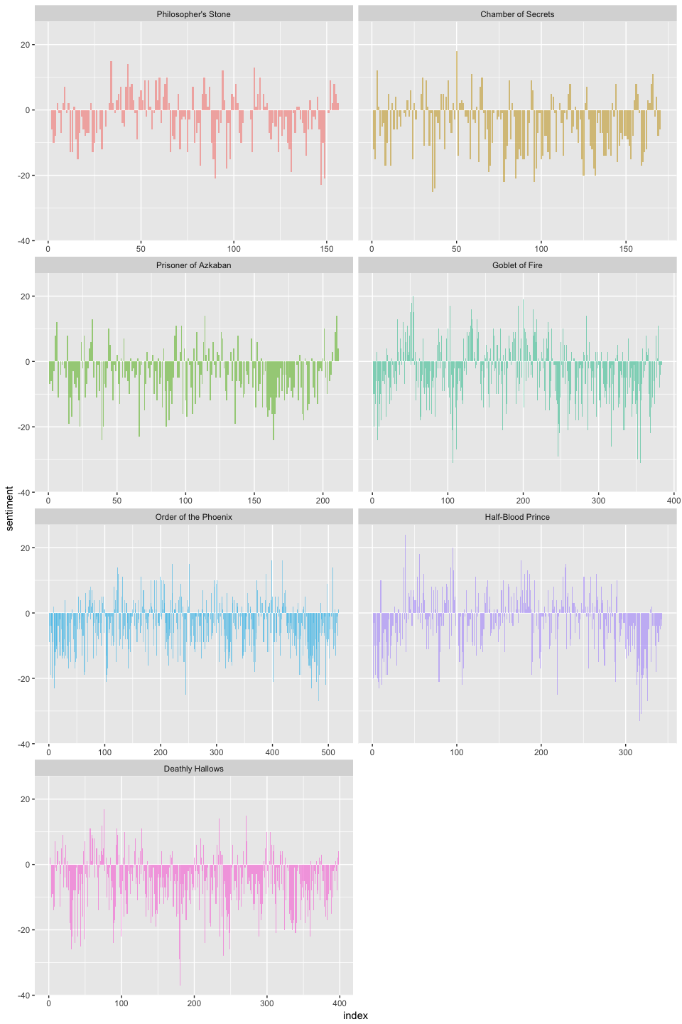
Now we can see how the plot of each novel changes toward more positive or negative sentiment over the trajectory of the story.
With several options for sentiment lexicons, you might want some more information on which one is appropriate for your purposes. Lets use all three sentiment lexicons and examine how they differ for each novel.
afinn <- series %>%
        group_by(book) %>%
        mutate(word_count = 1:n(),
               index = word_count %/% 500 + 1) %>%
        inner_join(get_sentiments("afinn")) %>%
        group_by(book, index) %>%
        summarise(sentiment = sum(score)) %>%
        mutate(method = "AFINN")

bing_and_nrc <- bind_rows(series %>%
                  group_by(book) %>%
                  mutate(word_count = 1:n(),
                         index = word_count %/% 500 + 1) %>%
                  inner_join(get_sentiments("bing")) %>%
                  mutate(method = "Bing"),
          series %>%
                  group_by(book) %>%
                  mutate(word_count = 1:n(),
                         index = word_count %/% 500 + 1) %>%
                  inner_join(get_sentiments("nrc") %>%
                                     filter(sentiment %in% c("positive", "negative"))) %>%
                  mutate(method = "NRC")) %>%
        count(book, method, index = index , sentiment) %>%
        ungroup() %>%
        spread(sentiment, n, fill = 0) %>%
        mutate(sentiment = positive - negative) %>%
        select(book, index, method, sentiment)
We now have an estimate of the net sentiment (positive - negative) in each chunk of the novel text for each sentiment lexicon. Let’s bind them together and plot them.
bind_rows(afinn,
          bing_and_nrc) %>%
        ungroup() %>%
        mutate(book = factor(book, levels = titles)) %>%
  ggplot(aes(index, sentiment, fill = method)) +
  geom_bar(alpha = 0.8, stat = "identity", show.legend = FALSE) +
  facet_grid(book ~ method)
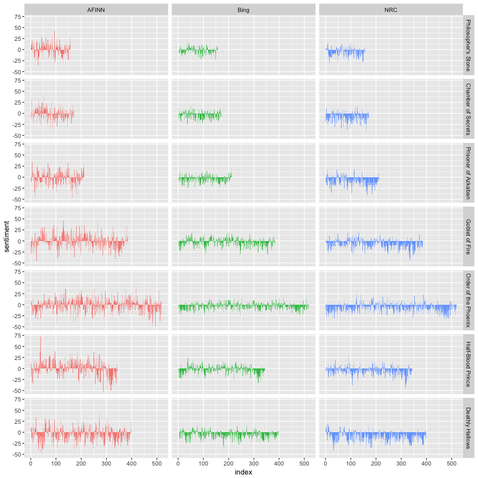
The three different lexicons for calculating sentiment give results that are different in an absolute sense but have fairly similar relative trajectories through the novels. We see similar dips and peaks in sentiment at about the same places in the novel, but the absolute values are significantly different. In some instances, it apears the AFINN lexicon finds more positive sentiments than the NRC lexicon. This output also allows us to compare across novels. First, you get a good sense of differences in book lengths - Order of the Pheonix is much longer than Philosopher’s Stone. Second, you can compare how books differ in their sentiment (both direction and magnitude) across a series.
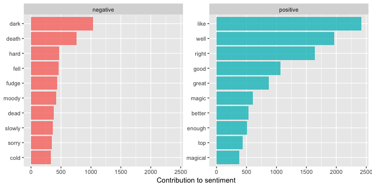
One advantage of having the data frame with both sentiment and word is that we can analyze word counts that contribute to each sentiment.
bing_word_counts <- series %>%
  inner_join(get_sentiments("bing")) %>%
  count(word, sentiment, sort = TRUE) %>%
  ungroup()

bing_word_counts
## # A tibble: 3,313 × 3
##      word sentiment     n
##     <chr>     <chr> <int>
## 1    like  positive  2416
## 2    well  positive  1969
## 3   right  positive  1643
## 4    good  positive  1065
## 5    dark  negative  1034
## 6   great  positive   877
## 7   death  negative   757
## 8   magic  positive   606
## 9  better  positive   533
## 10 enough  positive   509
## # ... with 3,303 more rows
We can view this visually to assess the top n words for each sentiment:
bing_word_counts %>%
        group_by(sentiment) %>%
        top_n(10) %>%
        ggplot(aes(reorder(word, n), n, fill = sentiment)) +
          geom_bar(alpha = 0.8, stat = "identity", show.legend = FALSE) +
          facet_wrap(~sentiment, scales = "free_y") +
          labs(y = "Contribution to sentiment", x = NULL) +
          coord_flip()
## Selecting by n
Lots of useful work can be done by tokenizing at the word level, but sometimes it is useful or necessary to look at different units of text. For example, some sentiment analysis algorithms look beyond only unigrams (i.e. single words) to try to understand the sentiment of a sentence as a whole. These algorithms try to understand that
I am not having a good day.
is a sad sentence, not a happy one, because of negation. The Stanford CoreNLP tools and the sentimentr R package (currently available on Github but not CRAN) are examples of such sentiment analysis algorithms. For these, we may want to tokenize text into sentences. I’ll illustrate using the philosophers_stone data set.
tibble(text = philosophers_stone) %>%
  unnest_tokens(sentence, text, token = "sentences")
## # A tibble: 6,598 × 1
##                                                                       sentence
##                                                                          <chr>
## 1                                              the boy who lived  mr. and mrs.
## 2  dursley, of number four, privet drive, were proud to say that they were per
## 3  they were the last people you'd expect to be involved in anything strange o
## 4                                                                          mr.
## 5      dursley was the director of a firm called grunnings, which made drills.
## 6  he was a big, beefy man with hardly any neck, although he did have a very l
## 7                                                                         mrs.
## 8  dursley was thin and blonde and had nearly twice the usual amount of neck,
## 9  the dursleys had a small son called dudley and in their opinion there was n
## 10 the dursleys had everything they wanted, but they also had a secret, and th
## # ... with 6,588 more rows
The argument token = "sentences" attempts to break up text by punctuation. Note how “mr.” and “mrs.” was placed on their own line. For most text this will have little impact but it is important to be aware of. You can also unnest text by “ngrams”, “lines”, “paragraphs”, and even using “regex”. Check out ?unnest_tokens for more details.
Lets go ahead and break up the philosophers_stone text by chapter and sentence.
ps_sentences <- tibble(chapter = 1:length(philosophers_stone),
                        text = philosophers_stone) %>%
  unnest_tokens(sentence, text, token = "sentences")
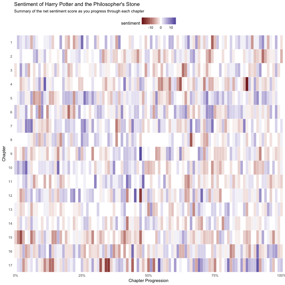
This will allow us to assess the net sentiment by chapter and by sentence. First, we need to track the sentence numbers and then I create an index that tracks the progress through each chapter. I then unnest the sentences by words. This gives us a tibble that has individual words by sentence within each chapter. Now, as before, I join the AFINN lexicon and compute the net sentiment score for each chapter. We can see that the most positive sentences are half way through chapter 9, towards the end of chapter 17, early in chapter 4, etc.
book_sent <- ps_sentences %>%
        group_by(chapter) %>%
        mutate(sentence_num = 1:n(),
               index = round(sentence_num / n(), 2)) %>%
        unnest_tokens(word, sentence) %>%
        inner_join(get_sentiments("afinn")) %>%
        group_by(chapter, index) %>%
        summarise(sentiment = sum(score, na.rm = TRUE)) %>%
        arrange(desc(sentiment))

book_sent
## Source: local data frame [1,401 x 3]
## Groups: chapter [17]
##
##    chapter index sentiment
##      <int> <dbl>     <int>
## 1        9  0.47        14
## 2       17  0.91        13
## 3        4  0.11        12
## 4       12  0.45        12
## 5       17  0.54        12
## 6        1  0.25        11
## 7       10  0.04        11
## 8       10  0.16        11
## 9       11  0.48        11
## 10      12  0.70        11
## # ... with 1,391 more rows
We can visualize this with a heatmap that shows the most positive and negative sentiments as we progress through each chapter
ggplot(book_sent, aes(index, factor(chapter, levels = sort(unique(chapter), decreasing = TRUE)), fill = sentiment)) +
        geom_tile(color = "white") +
        scale_fill_gradient2() +
        scale_x_continuous(labels = scales::percent, expand = c(0, 0)) +
        scale_y_discrete(expand = c(0, 0)) +
        labs(x = "Chapter Progression", y = "Chapter") +
        ggtitle("Sentiment of Harry Potter and the Philosopher's Stone",
                subtitle = "Summary of the net sentiment score as you progress through each chapter") +
        theme_minimal() +
        theme(panel.grid.major = element_blank(),
              panel.grid.minor = element_blank(),
              legend.position = "top")