
 Exponential forecasting is another smoothing method and has been around since the 1950s. Where niave forecasting places 100% weight on the most recent observation and moving averages place equal weight on k values, exponential smoothing allows for weighted averages where greater weight can be placed on recent observations and lesser weight on older observations. Exponential smoothing methods are intuitive, computationally efficient, and generally applicable to a wide range of time series. Consequently, exponentially smoothing is a great forecasting tool to have and this tutorial will walk you through the basics.
This tutorial primarily uses the fpp2 package. fpp2 will automatically load the forecast package (among others), which provides many of the key forecasting functions used throughout.
library(tidyverse)
library(fpp2)
Furthermore, we’ll use a couple data sets to illustrate. The goog and qcement data are provided by the fpp2 package. Let’s go ahead and set up training and validation sets:
# create training and validation of the Google stock data
goog.train <- window(goog, end = 900)
goog.test <- window(goog, start = 901)

# create training and validation of the AirPassengers data
qcement.train <- window(qcement, end = c(2012, 4))
qcement.test <- window(qcement, start = c(2013, 1))
The simplest of the exponentially smoothing methods is called “simple exponential smoothing” (SES). The key point to remember is that SES is suitable for data with no trend or seasonal pattern. This section will illustrate why.
For exponential smoothing, we weigh the recent observations more heavily than older observations. The weight of each observation is determined through the use of a smoothing parameter, which we will denote . For a data set with observations, we calculate our predicted value, , which will be based on through as follows:
where . It is also common to come to use the component form of this model, which uses the following set of equations.
In both equations we can see that the most weight is placed on the most recent observation. In practice, equal to 0.1-0.2 tends to perform quite well but we’ll demonstrate shortly how to tune this parameter. When is closer to 0 we consider this slow learning because the algorithm gives historical data more weight. When is closer to 1 we consider this fast learning because the algorithm gives more weight to the most recent observation; therefore, recent changes in the data will have a bigger impact on forecasted values. The following table illustrates how weighting changes based on the parameter:
| Observation | $$\alpha=0.2$$ | $$\alpha=0.4$$ | $$\alpha=0.6$$ | $$\alpha=0.8$$ |
|---|---|---|---|---|
| $$y_t$$ | 0.2 | 0.4 | 0.6 | 0.8 |
| $$y_{t-1}$$ | 0.16 | 0.24 | 0.26 | 0.16 |
| $$y_{t-2}$$ | 0.128 | 0.144 | 0.096 | 0.032 |
| $$y_{t-3}$$ | 0.1024 | 0.0864 | 0.0384 | 0.0064 |
| $$\vdots$$ | $$\vdots$$ | $$\vdots$$ | $$\vdots$$ | $$\vdots$$ |
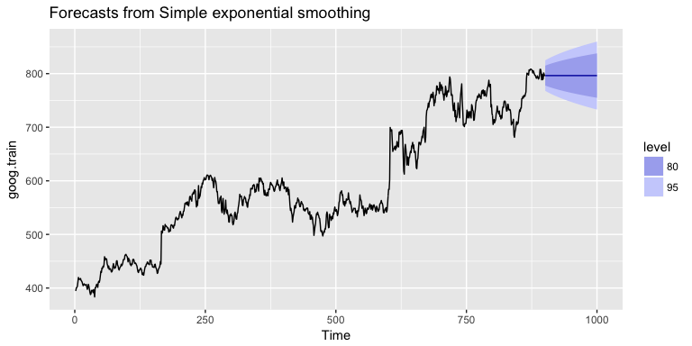
Let’s go ahead and apply SES to the Google data using the ses function. We manually set the for our initial model and forecast forward 100 steps with . We see that our forecast projects a flatlined estimate into the future, which does not capture the positive trend in the data. This is why SES should not be used on data with a trend or seasonal component.
ses.goog <- ses(goog.train, alpha = .2, h = 100)
autoplot(ses.goog)
One approach to correct for this is to difference our data to remove the trend. Now, goog.dif represents the change in stock price from the previous day.
goog.dif <- diff(goog.train)
autoplot(goog.dif)
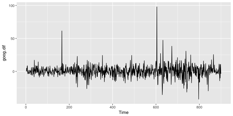
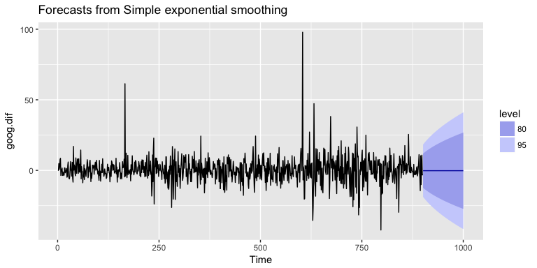
Once we’ve differenced we’ve effectively removed the trend from our data and can reapply the SES model.
ses.goog.dif <- ses(goog.dif, alpha = .2, h = 100)
autoplot(ses.goog.dif)
To understand how well the model predicts we can compare our forecasts to our validation data set. But first we need to create a differenced validation set since our training data was built on differenced data. We see that performance measures are smaller on the test set than the training so we are not overfitting our model.
goog.dif.test <- diff(goog.test)
accuracy(ses.goog.dif, goog.dif.test)
##                       ME     RMSE      MAE      MPE     MAPE      MASE
## Training set -0.01203526 9.467306 6.560186 112.0451 253.5440 0.7571417
## Test set      0.63032208 8.676901 6.341526 103.4038 103.4038 0.7319051
##                     ACF1 Theil's U
## Training set -0.05198282        NA
## Test set      0.16841378   1.01854
In our model we used the standard ; however, we can tune our alpha parameter to identify the value that reduces our forecasting error. Here we loop through alpha values from 0.01-0.99 and identify the level that minimizes our test RMSE. Turns out that minimizes our prediction error.
# identify optimal alpha parameter
alpha <- seq(.01, .99, by = .01)
RMSE <- NA
for(i in seq_along(alpha)) {
  fit <- ses(goog.dif, alpha = alpha[i], h = 100)
  RMSE[i] <- accuracy(fit, goog.dif.test)[2,2]
}

# convert to a data frame and idenitify min alpha value
alpha.fit <- data_frame(alpha, RMSE)
alpha.min <- filter(alpha.fit, RMSE == min(RMSE))

# plot RMSE vs. alpha
ggplot(alpha.fit, aes(alpha, RMSE)) +
  geom_line() +
  geom_point(data = alpha.min, aes(alpha, RMSE), size = 2, color = "blue")
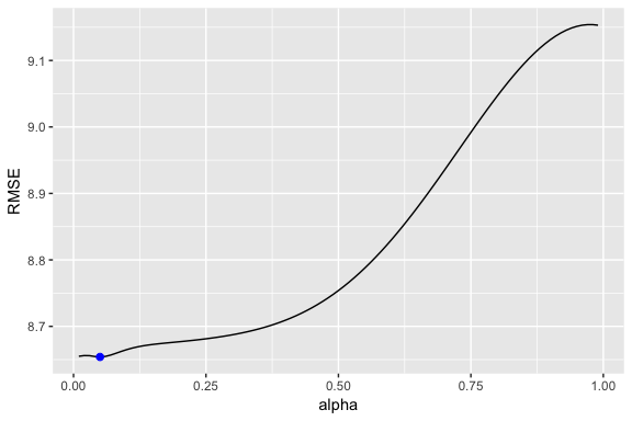
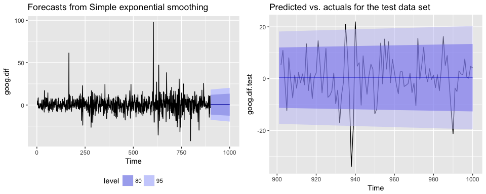
Now we can re-fit out SES with . Our performance metrics are not significantly different from our model where ; however, you will notice that the predicted confidence intervals are narrower (left chart). And when we zoom into the predicted versus actuals (right chart) you see that for most observations, our predicted confidence intervals did well.
# refit model with alpha = .05
ses.goog.opt <- ses(goog.dif, alpha = .05, h = 100)

# performance eval
accuracy(ses.goog.opt, goog.dif.test)
##                        ME     RMSE      MAE       MPE     MAPE      MASE
## Training set -0.005965793 9.088108 6.187613 116.75670 158.7963 0.7141413
## Test set      0.002419984 8.653976 6.297980  94.29215 102.7317 0.7268792
##                    ACF1 Theil's U
## Training set 0.01712706        NA
## Test set     0.16841378 0.9790798

# plotting results
p1 <- autoplot(ses.goog.opt) +
  theme(legend.position = "bottom")
p2 <- autoplot(goog.dif.test) +
  autolayer(ses.goog.opt, alpha = .5) +
  ggtitle("Predicted vs. actuals for the test data set")

gridExtra::grid.arrange(p1, p2, nrow = 1)
As mentioned and observed in the previous section, SES does not perform well with data that has a long-term trend. In the last section we illustrated how you can remove the trend with differencing and then perform SES. An alternative method to apply exponential smoothing while capturing trend in the data is to use Holt’s Method.
Holt’s Method makes predictions for data with a trend using two smoothing parameters, and , which correspond to the level and trend components, respectively. For Holt’s method, the prediction will be a line of some non-zero slope that extends from the time step after the last collected data point onwards.
The methodology for predictions using data with a trend (Holt’s Method) uses the following equation with observations. The k-step-ahead forecast is given by combining the level estimate at time t () and the trend estimate (which in this example is assumbed additive) at time t ().
The level () and trend () are updated through a pair of updating equations, which is where you see the presence of the two smoothing paramters:
In these equations, the first means that the level at time t is a weighted average of the actual value at time t and the level in the previous period, adjusted for trend. The second equation means that the trend at time t is a weighted average of the trend in the previous period and the more recent information on the change in the level. Similar to SES, and are constrained to 0-1 with higher values giving faster learning and lower values providing slower learning.
To capture a multiplicative (exponential) trend we make a minor adjustment in the above equations:
Holt’s method also has the alternative Component Form operations. In this case these represent the additive trend component form:
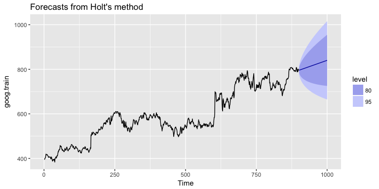
If we go back to our Google stock data, we can apply Holt’s method in the following manner. Here, we will not manually set the and for our initial model and forecast forward 100 steps with . We see that our forecast now does a better job capturing the positive trend in the data.
holt.goog <- holt(goog.train, h = 100)
autoplot(holt.goog)
Within holt you can manually set the and parameters; however, if you leave those parameters as NULL, the holt function will actually identify the optimal model parameters. It does this by minimizing AIC and BIC values. We can see the model selected by holt. In this case, meaning fast learning in the day-to-day movements and which means slow learning for the trend.
holt.goog$model
## Holt's method
##
## Call:
##  holt(y = goog.train, h = 100)
##
##   Smoothing parameters:
##     alpha = 0.9967
##     beta  = 1e-04
##
##   Initial states:
##     l = 395.991
##     b = 0.4484
##
##   sigma:  8.9383
##
##      AIC     AICc      BIC
## 10074.78 10074.85 10098.79
Let’s check the predictive accuracy of our model. According to our MAPE we have about a 2% error rate.
accuracy(holt.goog, goog.test)
##                        ME      RMSE       MAE         MPE     MAPE
## Training set -0.003922069  8.938319  5.974921 -0.01188414 1.004290
## Test set     -8.945342029 21.099897 16.268344 -1.15371296 2.039945
##                   MASE       ACF1 Theil's U
## Training set 0.9997514 0.03746482        NA
## Test set     2.7220944 0.89540070  2.481272
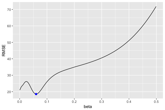
Similar to SES, we can tune the parameter to see if we can improve our predictive accuracy. The holt function identified an optimal ; however, this optimal value is based on minimizing errors on the training set, not minimizing prediction errors on the test set. Let’s assess a tradespace of values and see if we gain some predictive accuracy. Here, we loop through a series of values starting at 0.0001 all the way up to 0.5. We see that there is a dip in our RMSE at 0.0601.
# identify optimal alpha parameter
beta <- seq(.0001, .5, by = .001)
RMSE <- NA
for(i in seq_along(beta)) {
  fit <- holt(goog.train, beta = beta[i], h = 100)
  RMSE[i] <- accuracy(fit, goog.test)[2,2]
}

# convert to a data frame and idenitify min alpha value
beta.fit <- data_frame(beta, RMSE)
beta.min <- filter(beta.fit, RMSE == min(RMSE))

# plot RMSE vs. alpha
ggplot(beta.fit, aes(beta, RMSE)) +
  geom_line() +
  geom_point(data = beta.min, aes(beta, RMSE), size = 2, color = "blue")
Now let’s refit our model with this optimal value and compare our predictive accuracy to our original model. We see that our new model reduces our error rate (MAPE) down to 1.78%.
# new model with optimal beta
holt.goog.opt <- holt(goog.train, h = 100, beta = 0.0601)

# accuracy of first model
accuracy(holt.goog, goog.test)
##                        ME      RMSE       MAE         MPE     MAPE
## Training set -0.003922069  8.938319  5.974921 -0.01188414 1.004290
## Test set     -8.945342029 21.099897 16.268344 -1.15371296 2.039945
##                   MASE       ACF1 Theil's U
## Training set 0.9997514 0.03746482        NA
## Test set     2.7220944 0.89540070  2.481272

# accuracy of new optimal model
accuracy(holt.goog.opt, goog.test)
##                       ME      RMSE       MAE         MPE     MAPE     MASE
## Training set -0.01098347  9.109332  6.218278 -0.00502392 1.043517 1.040471
## Test set     -0.33180592 18.536622 14.287508 -0.09452438 1.780052 2.390652
##                    ACF1 Theil's U
## Training set 0.01293146        NA
## Test set     0.88797970  2.156113
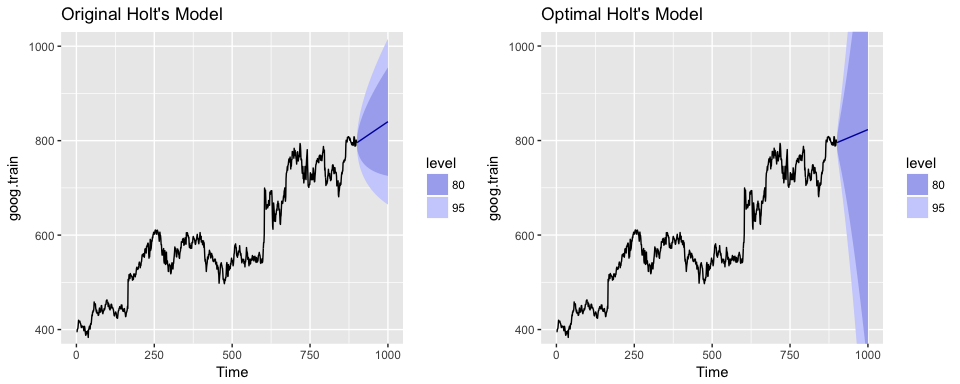
If we plot our original versus more recent optimal model we’ll notice a couple things. First, our predicted values for the optimal model are more conservative; in other words they are assuming a more gradual slope. Second, the confidence intervals are much more extreme. So although our predictions were more accurate, our uncertainty increases. The reason for this is that by increasing our value we are assuming faster learning from more recent observations. And since there some quite a bit of turbulence in the recent time period, this is causing greater variance to be incorporated into our prediction intervals. This requires a more indepth discussion than this tutorial will go into, but the important thing to keep in mind is that although we increase our prediction accuracy with parameter tuning, there are additional side effects that can occur, which may be harder to explain to decision-makers.
p1 <- autoplot(holt.goog) +
  ggtitle("Original Holt's Model") +
  coord_cartesian(ylim = c(400, 1000))

p2 <- autoplot(holt.goog.opt) +
  ggtitle("Optimal Holt's Model") +
  coord_cartesian(ylim = c(400, 1000))

gridExtra::grid.arrange(p1, p2, nrow = 1)
To make predictions using data with a trend and seasonality, we turn to the Holt-Winters Seasonal Method. This method can be implemented with an “Additive” structure or a “Multiplicative” structure, where the choice of method depends on the data set. The Additive model is best used when the seasonal trend is of the same magnitude throughout the data set, while the Multiplicative Model is preferred when the magnitude of seasonality changes as time increases.
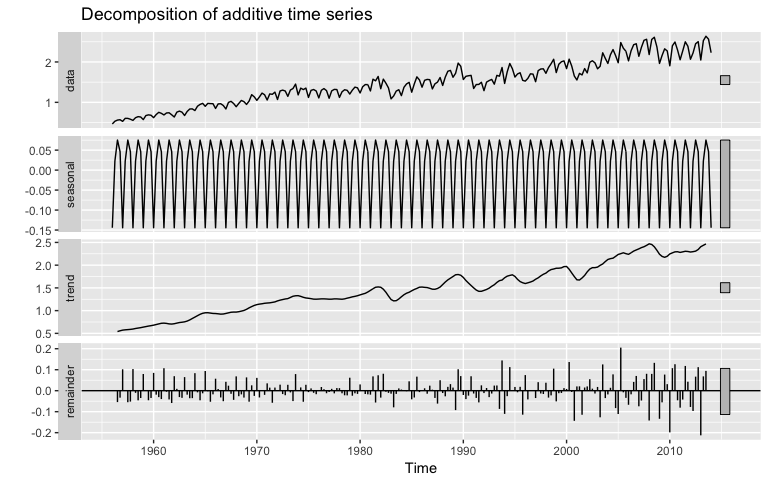
Since the Google data does not have seasonality, we’ll use the qcement data that we set up in the Replication section to demonstrate. This data has seasonality and trend; however, it is unclear if seasonality is additive or multiplicative. We’ll use the Holt-Winters method to identify the best fit model.
autoplot(decompose(qcement))
For the Additive model, the regular equation form is:
The level (), trend (), and season () are updated through a pair of updating equations, which is where you see the presence of the three smoothing paramters:
where , , and are the three smoothing parameters to deal with the level pattern, the trend, and the seasonality, respectively. Similar to SES and Holt’s method, all three parameters are constrained to 0-1. The component equations are as follows:
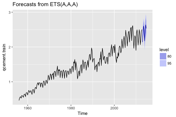
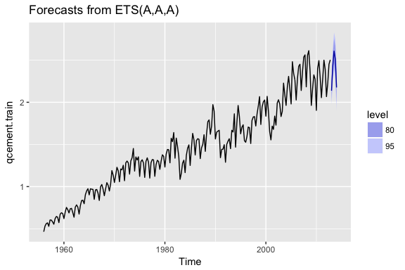
To apply the Holt-Winters method we’ll introduce a new function, ets which stands for error, trend, and seasonality. The important thing to understand about the ets model is how to select the model = parameter. In total you have 36 model options to choose from. The parameter settings in the below code (model = "AAA") stands for a model with additive error, additive trend, and additve seasonality.
qcement.hw <- ets(qcement.train, model = "AAA")
autoplot(forecast(qcement.hw))
So when specificying the model type you always specificy the error, trend, then seasonality (hence “ets”). The options you can specify for each component is as follows:
Consequently, if you wanted to apply a Holt’s model where the error and trend were additive and no seasonality exists you would select model = "AAN". If you want to apply a Holt-Winters model where there is additive error, an exponential (multiplicative) trend, and additive seasonality you would select model = "AMA". If you are uncertain of the type of component then you use “Z”. So if you were uncertain of the components or if you want the model to select the best option, you could use model = "ZZZ" and the “optimal” model will be selected.
If we assess our additive model we can see that , , and
summary(qcement.hw)
## ETS(A,A,A)
##
## Call:
##  ets(y = qcement.train, model = "AAA")
##
##   Smoothing parameters:
##     alpha = 0.6208
##     beta  = 1e-04
##     gamma = 0.1913
##
##   Initial states:
##     l = 0.4969
##     b = 0.0086
##     s=5e-04 0.0357 0.02 -0.0562
##
##   sigma:  0.0838
##
##      AIC     AICc      BIC
## 125.0495 125.8752 155.9136
##
## Training set error measures:
##                         ME       RMSE        MAE        MPE     MAPE
## Training set -0.0004297096 0.08375033 0.05912561 -0.1834617 3.830243
##                   MASE       ACF1
## Training set 0.5849367 0.04576105
If we check our residuals, we see that residuals grow larger over time. This may suggest that a multiplicative error rate may be more appropriate.
checkresiduals(qcement.hw)
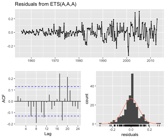
##
## 	Ljung-Box test
##
## data:  Residuals from ETS(A,A,A)
## Q* = 21.863, df = 3, p-value = 6.965e-05
##
## Model df: 8.   Total lags used: 11
If we check the predictive accuracy we see that our prediction accuracy is about 2.9% (according to the MAPE).
# forecast the next 5 quarters
qcement.f1 <- forecast(qcement.hw, h = 5)

# check accuracy
accuracy(qcement.f1, qcement.test)
##                         ME       RMSE        MAE        MPE     MAPE
## Training set -0.0004297096 0.08375033 0.05912561 -0.1834617 3.830243
## Test set      0.0307206913 0.07102359 0.06762179  1.0818090 2.882741
##                   MASE        ACF1 Theil's U
## Training set 0.5849367  0.04576105        NA
## Test set     0.6689904 -0.30067586 0.2084824
As previously stated, we may have multiplicative features for our Holt-Winters method. If we have multiplicative seasonality then our equation form changes to:
The level (), trend (), and season () are updated through a pair of updating equations, which is where you see the presence of the three smoothing paramters:
If we apply a multiplicative seasonality model then our model parameter becomes model = "MAM" (here, we are actually applying a multiplicative error and seasonality model). We see that are residuals illustrate less change in magnitude over time. We still have an issue with autocorrelation with errors but we’ll address that in later tutorials.
qcement.hw2 <- ets(qcement.train, model = "MAM")
checkresiduals(qcement.hw2)
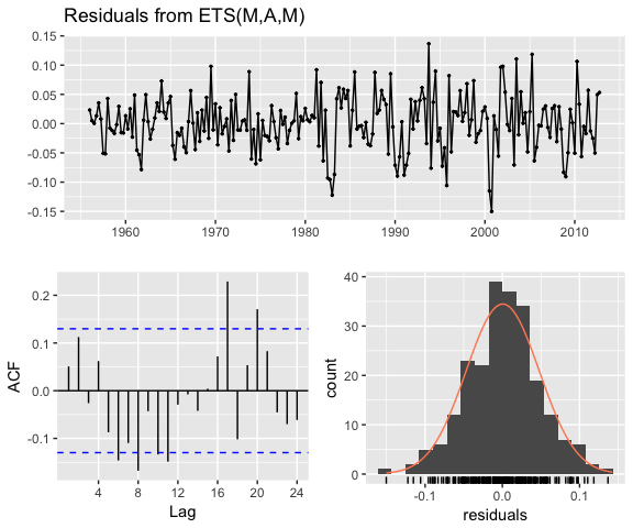
##
## 	Ljung-Box test
##
## data:  Residuals from ETS(M,A,M)
## Q* = 31.054, df = 3, p-value = 8.28e-07
##
## Model df: 8.   Total lags used: 11
To compare the predictive accuracy of our models let’s compare four different models. We see that the first model (additive error, trend and seasonality) results in the lowest RMSE and MAPE on our test data set.
# additive error, trend and seasonality
qcement.hw1 <- ets(qcement.train, model = "AAA")
qcement.f1 <- forecast(qcement.hw1, h = 5)
accuracy(qcement.f1, qcement.test)
##                         ME       RMSE        MAE        MPE     MAPE
## Training set -0.0004297096 0.08375033 0.05912561 -0.1834617 3.830243
## Test set      0.0307206913 0.07102359 0.06762179  1.0818090 2.882741
##                   MASE        ACF1 Theil's U
## Training set 0.5849367  0.04576105        NA
## Test set     0.6689904 -0.30067586 0.2084824

# multiplicative error, additive trend and seasonality
qcement.hw2 <- ets(qcement.train, model = "MAA")
qcement.f2 <- forecast(qcement.hw2, h = 5)
accuracy(qcement.f2, qcement.test)
##                      ME       RMSE        MAE       MPE     MAPE      MASE
## Training set 0.00865174 0.08430224 0.06016351 0.3681282 3.855631 0.5952048
## Test set     0.05325330 0.08920858 0.08787368 2.0147773 3.704400 0.8693447
##                     ACF1 Theil's U
## Training set  0.02351973        NA
## Test set     -0.18115593 0.2782566

# additive error and trend and multiplicative seasonality
qcement.hw3 <- ets(qcement.train, model = "AAM", restrict = FALSE)
qcement.f3 <- forecast(qcement.hw3, h = 5)
accuracy(qcement.f3, qcement.test)
##                       ME       RMSE       MAE       MPE     MAPE      MASE
## Training set 0.003403387 0.07762833 0.0558983 0.1487162 3.693408 0.5530085
## Test set     0.027648352 0.08382395 0.0777908 0.8568631 3.304030 0.7695936
##                     ACF1 Theil's U
## Training set -0.02009013        NA
## Test set     -0.06590551 0.2161475

# multiplicative error, additive trend, and multiplicative seasonality
qcement.hw4 <- ets(qcement.train, model = "MAM")
qcement.f4 <- forecast(qcement.hw4, h = 5)
accuracy(qcement.f4, qcement.test)
##                         ME       RMSE        MAE        MPE     MAPE
## Training set -0.0002168053 0.07890496 0.05632428 -0.1768320 3.674397
## Test set      0.0254950165 0.08572543 0.07730926  0.7486433 3.277401
##                   MASE        ACF1 Theil's U
## Training set 0.5572228  0.04834983        NA
## Test set     0.7648297 -0.05507385 0.2188327
If we were to compare this to an unspecified model where we let ets select the optimal model, we see that ets selects a model specification of multiplicative error, additive trend, and multiplicative seasonality (“MAM”). This is equivalent to our fourth model above. This model is assumed “optimal” because it minimizes RMSE, AIC, and BIC on the training data set, but does not necessarily minimize prediction errors on the test set.
qcement.hw5 <- ets(qcement.train, model = "ZZZ")
summary(qcement.hw5)
## ETS(M,A,M)
##
## Call:
##  ets(y = qcement.train, model = "ZZZ")
##
##   Smoothing parameters:
##     alpha = 0.693
##     beta  = 0.0261
##     gamma = 1e-04
##
##   Initial states:
##     l = 0.4899
##     b = 0.0114
##     s=1.0291 1.0487 1.0157 0.9064
##
##   sigma:  0.0473
##
##       AIC      AICc       BIC
##  4.569915  5.395603 35.434025
##
## Training set error measures:
##                         ME       RMSE        MAE       MPE     MAPE
## Training set -0.0002168053 0.07890496 0.05632428 -0.176832 3.674397
##                   MASE       ACF1
## Training set 0.5572228 0.04834983
As we did in the SES and Holt’s method section, we can optimize the parameter in our Holt-Winters model. Here, we use the additive error, trend and seasonality model that minimized our prediction errors above and identify the parameter that minimizes forecast errors. In this case we see that minimizes the error rate.
gamma <- seq(0.01, 0.85, 0.01)
RMSE <- NA

for(i in seq_along(gamma)) {
  hw.expo <- ets(qcement.train, "AAA", gamma = gamma[i])
  future <- forecast(hw.expo, h = 5)
  RMSE[i] = accuracy(future, qcement.test)[2,2]
}

error <- data_frame(gamma, RMSE)
minimum <- filter(error, RMSE == min(RMSE))
ggplot(error, aes(gamma, RMSE)) +
  geom_line() +
  geom_point(data = minimum, color = "blue", size = 2) +
  ggtitle("gamma's impact on forecast errors",
          subtitle = "gamma = 0.21 minimizes RMSE")
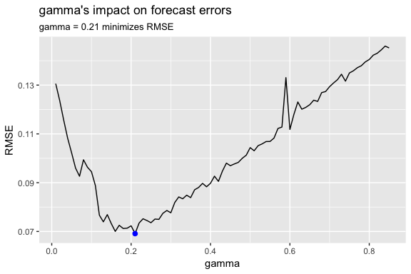
If we update our model with this “optimal” parameter we see that we bring our forecasting error rate down from 2.88% to 2.76%. This is a small improvement, but often small improvements can have large business implications.
# previous model with additive error, trend and seasonality
accuracy(qcement.f1, qcement.test)
##                         ME       RMSE        MAE        MPE     MAPE
## Training set -0.0004297096 0.08375033 0.05912561 -0.1834617 3.830243
## Test set      0.0307206913 0.07102359 0.06762179  1.0818090 2.882741
##                   MASE        ACF1 Theil's U
## Training set 0.5849367  0.04576105        NA
## Test set     0.6689904 -0.30067586 0.2084824

# new model with optimal gamma parameter
qcement.hw6 <- ets(qcement.train, model = "AAA", gamma = 0.21)
qcement.f6 <- forecast(qcement.hw6, h = 5)
accuracy(qcement.f6, qcement.test)
##                        ME       RMSE        MAE       MPE     MAPE
## Training set -0.001206215 0.08425184 0.05975069 -0.154495 3.974104
## Test set      0.029358296 0.06911376 0.06466821  1.038366 2.761642
##                   MASE        ACF1 Theil's U
## Training set 0.5911206  0.03804556        NA
## Test set     0.6397703 -0.36727559 0.2081361
With this new optimal model we can get our predicted values:
qcement.f6
##         Point Forecast    Lo 80    Hi 80    Lo 95    Hi 95
## 2013 Q1       2.137275 2.029302 2.245248 1.972144 2.302405
## 2013 Q2       2.431710 2.304338 2.559081 2.236912 2.626507
## 2013 Q3       2.607007 2.462819 2.751194 2.386491 2.827523
## 2013 Q4       2.509414 2.350171 2.668657 2.265873 2.752954
## 2014 Q1       2.175803 1.992753 2.358854 1.895852 2.455755
and also visualize these predicted values:
autoplot(qcement.f6)
One last item to discuss is the idea of “damping” your forecast. Damped forecasts use a damping coefficient denoted to more conservatively estimate the predicted trend. Basically, if you believe that your additive or multiplicative trend is or will be slowing down (“flat-lining”) in the near future then you are assuming it will dampen.
The equation form for an additive model with a damping coefficient is
where . When the method is the same as Holt’s additive model. As gets closer to 0, the trend becomes more conservative and flat-lines to a constant in the nearer future. The end result of this method is that short-run forecasts are still trended while long-run forecasts are constant.
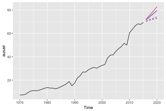
To illustrate the effect of a damped forecast we’ll use the fpp2::ausair data set. Here, we create several models (additive, additive + damped, multiplicative, multiplicative + damped). In the plot you can see that the damped models (dashed lines) have more conservative trend lines and if we forecasted these far enough into the future we would see this trend flat-line.
# holt's linear (additive) model
fit1 <- ets(ausair, model = "ZAN", alpha = 0.8, beta = 0.2)
pred1 <- forecast(fit1, h = 5)

# holt's linear (additive) model
fit2 <- ets(ausair, model = "ZAN", damped = TRUE, alpha = 0.8, beta = 0.2, phi = 0.85)
pred2 <- forecast(fit2, h = 5)

# holt's exponential (multiplicative) model
fit3 <- ets(ausair, model = "ZMN", alpha = 0.8, beta = 0.2)
pred3 <- forecast(fit3, h = 5)

# holt's exponential (multiplicative) model damped
fit4 <- ets(ausair, model = "ZMN", damped = TRUE, alpha = 0.8, beta = 0.2, phi = 0.85)
pred4 <- forecast(fit4, h = 5)

autoplot(ausair) +
  autolayer(pred1$mean, color = "blue") +
  autolayer(pred2$mean, color = "blue", linetype = "dashed") +
  autolayer(pred3$mean, color = "red") +
  autolayer(pred4$mean, color = "red", linetype = "dashed")
The above models were for illustrative purposes only. You would apply the same process as you saw in earlier sections to identify if a damped model predicts more accurately than a non-dampped model. You can even apply the approaches you saw earlier for tuning this parameter to identify the optimal coefficient.
Use the usmelec data set which is provided by the fpp2 package.