
So far we have focused on identifying the frequency of individual terms within a document along with the sentiments that these words provide. It is also important to understand the importance that words provide within and across documents. As we saw in the tidy text tutorial term frequency (tf) identifies how frequently a word occurs in a document. We found that many common words such as “the”, “is”, “for”, etc. typically top the term frequency lists. One approach to correct for these common, yet low context words, is to remove these words by using a list of stop words.
Another approach is to use what is called a term’s inverse document frequency (idf), which decreases the weight for commonly used words and increases the weight for words that are not used very much in a collection of documents. The idf is defined as:
where the idf of a given term (t) in a set of documents (D) is a function of the total number of documents being assessed (N) and the number of documents where the term t appears (). In addition, we can combine tf and idf statistics into a single tf-idf statistic, which computes the frequency of a term adjusted for how rarely it is used. Since the ratio inside the idf’s log function is always greater than or equal to 1, the value of idf (and tf-idf) is greater than or equal to 0. As a term appears in more documents, the ratio inside the logarithm approaches 1, bringing the idf and tf-idf closer to 0. tf-idf is defined as
where tf-idf for a particular term (t) in docuement (d) for a set of documents (D) is simply the product of that term’s tf and idf statistics. This tutorial will walk you through the process of computing these values so that you can identify high frequency words that provide particularly important context to a single document within a group of documents.
This tutorial builds on the tidy text and sentiment analysis tutorials so if you have not read through those tutorials I suggest you start there before proceeding. In this tutorial I cover the following:
This tutorial leverages the data provided in the harrypotter package. I constructed this package to supply the first seven novels in the Harry Potter series to illustrate text mining and analysis capabilities. You can load the harrypotter package with the following:
if (packageVersion("devtools") < 1.6) {
  install.packages("devtools")
}

devtools::install_github("bradleyboehmke/harrypotter")
library(tidyverse)      # data manipulation & plotting
library(stringr)        # text cleaning and regular expressions
library(tidytext)       # provides additional text mining functions
library(harrypotter)    # provides the first seven novels of the Harry Potter series
The seven novels we are working with, and are provided by the harrypotter package, include:
philosophers_stone: Harry Potter and the Philosophers Stone (1997)chamber_of_secrets: Harry Potter and the Chamber of Secrets (1998)prisoner_of_azkaban: Harry Potter and the Prisoner of Azkaban (1999)goblet_of_fire: Harry Potter and the Goblet of Fire (2000)order_of_the_phoenix: Harry Potter and the Order of the Phoenix (2003)half_blood_prince: Harry Potter and the Half-Blood Prince (2005)deathly_hallows: Harry Potter and the Deathly Hallows (2007)Each text is in a character vector with each element representing a single chapter. For instance, the following illustrates the raw text of the first two chapters of the philosophers_stone:
philosophers_stone[1:2]
## [1] "THE BOY WHO LIVED  Mr. and Mrs. Dursley, of number four, Privet Drive, were proud to say that they
## were perfectly normal, thank you very much. They were the last people you'd expect to be involved in anything
## strange or mysterious, because they just didn't hold with such nonsense.  Mr. Dursley was the director of a
## firm called Grunnings, which made drills. He was a big, beefy man with hardly any neck, although he did have a
## very large mustache. Mrs. Dursley was thin and blonde and had nearly twice the usual amount of neck, which came
## in very useful as she spent so much of her time craning over garden fences, spying on the neighbors. The
## Dursleys had a small son called Dudley and in their opinion there was no finer boy anywhere.  The Dursleys
## had everything they wanted, but they also had a secret, and their greatest fear was that somebody would
## discover it. They didn't think they could bear it if anyone found out about the Potters. Mrs. Potter was Mrs.
## Dursley's sister, but they hadn'... <truncated>
## [2] "THE VANISHING GLASS  Nearly ten years had passed since the Dursleys had woken up to find their nephew on
## the front step, but Privet Drive had hardly changed at all. The sun rose on the same tidy front gardens and lit
## up the brass number four on the Dursleys' front door; it crept into their living room, which was almost exactly
## the same as it had been on the night when Mr. Dursley had seen that fateful news report about the owls. Only
## the photographs on the mantelpiece really showed how much time had passed. Ten years ago, there had been lots
## of pictures of what looked like a large pink beach ball wearing different-colored bonnets -- but Dudley Dursley
## was no longer a baby, and now the photographs showed a large blond boy riding his first bicycle, on a carousel
## at the fair, playing a computer game with his father, being hugged and kissed by his mother. The room held no
## sign at all that another boy lived in the house, too.  Yet Harry Potter was still there, asleep at the
## moment, but no... <truncated>
To compute term frequencies we need to have our data in a tidy format. The following converts all seven Harry Potter novels into a tibble that has each word by chapter by book. See the tidy text tutorial for more details.
titles <- c("Philosopher's Stone", "Chamber of Secrets", "Prisoner of Azkaban",
            "Goblet of Fire", "Order of the Phoenix", "Half-Blood Prince",
            "Deathly Hallows")

books <- list(philosophers_stone, chamber_of_secrets, prisoner_of_azkaban,
           goblet_of_fire, order_of_the_phoenix, half_blood_prince,
           deathly_hallows)

series <- tibble()

for(i in seq_along(titles)) {

        clean <- tibble(chapter = seq_along(books[[i]]),
                        text = books[[i]]) %>%
             unnest_tokens(word, text) %>%
             mutate(book = titles[i]) %>%
             select(book, everything())

        series <- rbind(series, clean)
}

# set factor to keep books in order of publication
series$book <- factor(series$book, levels = rev(titles))

series
## # A tibble: 1,089,386 × 3
##                   book chapter    word
## *               <fctr>   <int>   <chr>
## 1  Philosopher's Stone       1     the
## 2  Philosopher's Stone       1     boy
## 3  Philosopher's Stone       1     who
## 4  Philosopher's Stone       1   lived
## 5  Philosopher's Stone       1      mr
## 6  Philosopher's Stone       1     and
## 7  Philosopher's Stone       1     mrs
## 8  Philosopher's Stone       1 dursley
## 9  Philosopher's Stone       1      of
## 10 Philosopher's Stone       1  number
## # ... with 1,089,376 more rows
From this cleaned up text we can compute the term frequency for each word. Lets do this for computing term frequencies by book and across the entire Harry Potter series:
book_words <- series %>%
        count(book, word, sort = TRUE) %>%
        ungroup()

series_words <- book_words %>%
        group_by(book) %>%
        summarise(total = sum(n))

book_words <- left_join(book_words, series_words)

book_words
## # A tibble: 67,881 × 4
##                    book  word     n  total
##                  <fctr> <chr> <int>  <int>
## 1  Order of the Phoenix   the 11740 258763
## 2       Deathly Hallows   the 10335 198906
## 3        Goblet of Fire   the  9305 191882
## 4     Half-Blood Prince   the  7508 171284
## 5  Order of the Phoenix    to  6518 258763
## 6  Order of the Phoenix   and  6189 258763
## 7       Deathly Hallows   and  5510 198906
## 8  Order of the Phoenix    of  5332 258763
## 9   Prisoner of Azkaban   the  4990 105275
## 10       Goblet of Fire   and  4959 191882
## # ... with 67,871 more rows
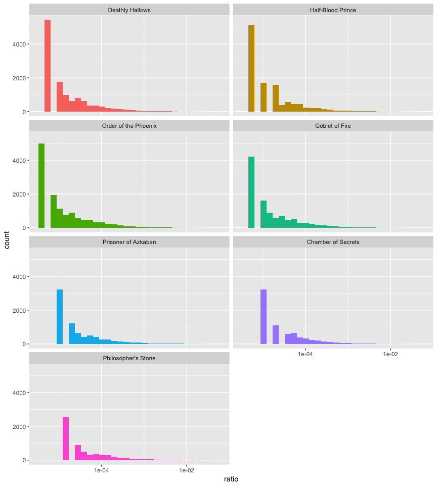
Here, we can see that common and noncontextual words (“the”, “to”, “and”, “of”, etc.) rule the term frequency list. We can visualize the distribution of term frequency for each novel. Here we’ll look at the distribution of n/total. Since the distribution is so clustered around 0 I add scale_x_log10() to spread it out. Even so we see the long right tails for thos extremely common words.
book_words %>%
        mutate(ratio = n / total) %>%
        ggplot(aes(ratio, fill = book)) +
        geom_histogram(show.legend = FALSE) +
        scale_x_log10() +
        facet_wrap(~ book, ncol = 2)
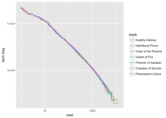
Zipf’s law states that within a group or corpus of documents, the frequency of any word is inversely proportional to its rank in a frequency table. Thus the most frequent word will occur approximately twice as often as the second most frequent word, three times as often as the third most frequent word, etc. Zipf’s law is most easily observed by plotting the data on a log-log graph, with the axes being log(rank order) and log(term frequency).
freq_by_rank <- book_words %>%
        group_by(book) %>%
        mutate(rank = row_number(),
               `term freq` = n / total)


ggplot(freq_by_rank, aes(rank, `term freq`, color = book)) +
        geom_line() +
        scale_x_log10() +
        scale_y_log10()
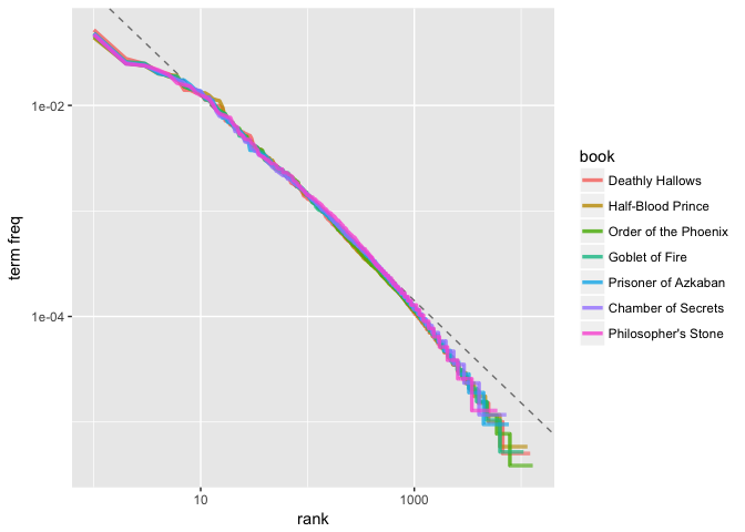
Our plot illustrates that the distribution is similar across the seven books. Furthermore, we can compare the distribution to a simple regression line. We see that the tails of the distribution deviate suggesting our distribution doesn’t follow Zipf’s law perfectly; however, it is close enough to generally state that the law approximately holds within our corpus of text.
lower_rank <- freq_by_rank %>%
        filter(rank < 500)

lm(log10(`term freq`) ~ log10(rank), data = lower_rank)
##
## Call:
## lm(formula = log10(`term freq`) ~ log10(rank), data = lower_rank)
##
## Coefficients:
## (Intercept)  log10(rank)
##     -0.9414      -0.9694

freq_by_rank %>%
        ggplot(aes(rank, `term freq`, color = book)) +
        geom_abline(intercept = -0.9414, slope = -0.9694, color = "gray50", linetype = 2) +
        geom_line(size = 1.2, alpha = 0.8) +
        scale_x_log10() +
        scale_y_log10()
The idea of tf-idf is to find the important words for the content of each document by decreasing the weight for commonly used words and increasing the weight for words that are not used very much in a collection or corpus of documents, in this case, the Harry Potter series. Calculating tf-idf attempts to find the words that are important (i.e., common) in a text, but not too common. Or put another way, tf-idf helps to find the important words that can provide specific document context. We can easily compute the idf and tf-idf using the bind_tf_idf function provided by the tidytext package.
book_words <- book_words %>%
        bind_tf_idf(word, book, n)

book_words
## # A tibble: 67,881 × 7
##                    book  word     n  total         tf   idf tf_idf
##                  <fctr> <chr> <int>  <int>      <dbl> <dbl>  <dbl>
## 1  Order of the Phoenix   the 11740 258763 0.04536970     0      0
## 2       Deathly Hallows   the 10335 198906 0.05195922     0      0
## 3        Goblet of Fire   the  9305 191882 0.04849334     0      0
## 4     Half-Blood Prince   the  7508 171284 0.04383363     0      0
## 5  Order of the Phoenix    to  6518 258763 0.02518907     0      0
## 6  Order of the Phoenix   and  6189 258763 0.02391764     0      0
## 7       Deathly Hallows   and  5510 198906 0.02770153     0      0
## 8  Order of the Phoenix    of  5332 258763 0.02060573     0      0
## 9   Prisoner of Azkaban   the  4990 105275 0.04739967     0      0
## 10       Goblet of Fire   and  4959 191882 0.02584401     0      0
## # ... with 67,871 more rows
Notice how the common non-contextual words (“the”, “to”, “and”, etc.) have high tf values but their idf and tf-idf values are 0. Remember that so these common terms that occur in every document will have an And since tf-idf is simply this will also be zero.
We can look at the words that have the highest tf-idf values. Here we see mainly names for characters in each book that are unique to that book, and therefore used often, but are absent or nearly absent in the other books.
book_words %>%
        arrange(desc(tf_idf))
## # A tibble: 67,881 × 7
##                    book        word     n  total           tf       idf
##                  <fctr>       <chr> <int>  <int>        <dbl>     <dbl>
## 1     Half-Blood Prince    slughorn   335 171284 0.0019558161 1.2527630
## 2       Deathly Hallows           c  1300 198906 0.0065357506 0.3364722
## 3  Order of the Phoenix    umbridge   496 258763 0.0019168119 0.8472979
## 4        Goblet of Fire      bagman   208 191882 0.0010839995 1.2527630
## 5    Chamber of Secrets    lockhart   197  85401 0.0023067646 0.5596158
## 6   Prisoner of Azkaban       lupin   369 105275 0.0035051057 0.3364722
## 7        Goblet of Fire       winky   145 191882 0.0007556728 1.2527630
## 8        Goblet of Fire   champions    84 191882 0.0004377690 1.9459101
## 9       Deathly Hallows xenophilius    79 198906 0.0003971725 1.9459101
## 10    Half-Blood Prince    mclaggen    65 171284 0.0003794867 1.9459101
## # ... with 67,871 more rows, and 1 more variables: tf_idf <dbl>
To understand the most common contextual words in each book we can take a look at the top 15 terms with the highest tf-idf.
book_words %>%
        arrange(desc(tf_idf)) %>%
        mutate(word = factor(word, levels = rev(unique(word))),
               book = factor(book, levels = titles)) %>%
        group_by(book) %>%
        top_n(15, wt = tf_idf) %>%
        ungroup() %>%
        ggplot(aes(word, tf_idf, fill = book)) +
        geom_bar(stat = "identity", alpha = .8, show.legend = FALSE) +
        labs(title = "Highest tf-idf words in the Harry Potter series",
             x = NULL, y = "tf-idf") +
        facet_wrap(~book, ncol = 2, scales = "free") +
        coord_flip()
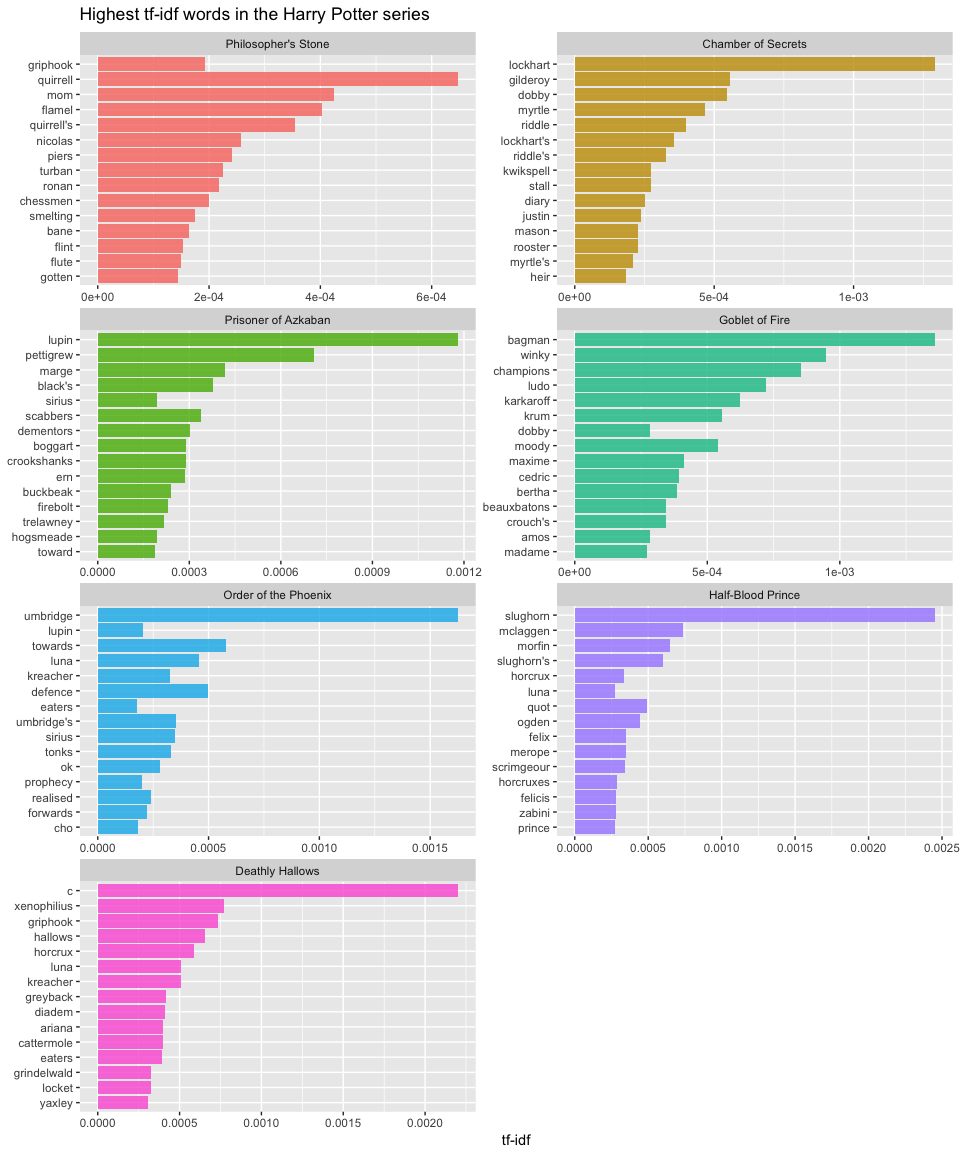
As you can see most of these high ranking tf-idf words are nouns that provide specific context around the the most common characters in each individual book.